advanced-pdes

[cinder marten]

so like, I can choose alternative coordinates, and expressing the laplacian in those different coordinates will still be the same differential operator as the global one, but only on the patch on which they are defined upon

a simpler example is the exterior derivative. I can express d locally as d/dx^i dx^i and solve locally for exact functions, but I have to piece them together to actually get a globally exact thing

this is where the topology of your manifold comes in

[gleaming lily]

Evans proves that $W^{1,p}(U)\subset\subset L^p(U)$ for $p<n$, and claims that for $p>n$ it follows from Morrey's inequality and Arzela Ascoli

[untold delta]

.whoever

[gleaming lily]

I don't see how this is the case

[gleaming lily]

Ok I see now

[gleaming lily]

Why does v_i exist in L^infty?

[lilac barn]

D^-h is bounded so it is bounded in L2 for any compact set uniformly in h. Now using that L2 is reflexive and a diagonalization argument, extract a subsequence of D-h which converges for all compact subsets. Finally, extract an a.e subsequence from this which ensures the almost sure bound.

[untold delta]

criver

criver

[buoyant pike]

I'm not sure but I don't think so

If you want to try searching online the keyword is "boundary integral method"

Oh actually I've changed my mind I think it is true

Oh nevermind I've changed my mind again

There is a normalizing factor in front but it doesn't scale the same way that the surface area of a sphere scales

Whatever just ignore me

[empty terrace]

I am pretty sure it is true, it always holds for all randomized numerical experiments I did

I think min-max would be violated if it were not true

Because then I can pick an f to make a point in the interior be larger or smaller than the points on the boundary

i.e. if w is not positive and integrating to 1 one the Dirichlet boundary

[buoyant pike]

Ok I believe that

[empty terrace]

Doesn't hold for biharmonic though I think, because there is no max-min principle there

i.e. it models plate bending, and the bend can happen in the middle of the domain, resulting in a max/min away from the boundary

[empty terrace]

Thing is I have never seen it formulated as such, so I was wondering whether there's a reference discussing this property of the Laplacian's Green's functions

[buoyant pike]

Boundary integral method literature probably

[empty terrace]

That's pretty sparse (at least from what I have found) when it comes to arbitrary mixed boundary conditions

The best I could find there was Melnikov's paper discussing Green's functions for a square boundary

[buoyant pike]

You don’t have a mixed boundary condition though?

[empty terrace]

I do, Г_N and Г_D

In fact the tests I did are for such a boundary, and the Г_D boundary is even fairly arbitrary (not a square)

[buoyant pike]

Oh wait they are not the same boundary?

[empty terrace]

Of course not

You can't prescribe both d_n u = 0 and u = f on the same boundary in general

[gleaming lily]

Weak convergence implies subsequence converging a.e.?

[lilac barn]

Nope

Well not in Lp. It does for continuous functions/uniform-convergence

[gleaming lily]

What do you mean?

[lilac barn]

If (X = C[0,1]) then ( f_n \rightharpoonup f \iff \sup_{n \in \mathbb{N}}\lVert f_n \rVert_{\infty} < \infty \land \forall x \in [0,1]: f_n(x) \xrightarrow{p.w.} f(x) ).

If (X = L^p[0,1], p \in (1,\infty)) then (f_n \rightharpoonup f \iff \sup_{n \in \mathbb{N}} \lVert f_n \rVert_{L^p} < \infty \land \forall x \in [0,1] : \int_{0}^x f_n \to \int_{0}^x f. )

[untold delta]

cocat

[lilac barn]

In particular, weak convergence implies a.e. convergence for continuous spaces but not for Lp space

Even more simply, if it did then Lp convergence implies weak convergence which would imply Lp convergence implies a.e. convergence which is false.

[gleaming lily]

But we only know weak convergence in L^2

Not weak convergence in the L^infty norm for C[0,1] right

[lilac barn]

Oh I did end up equivating weak and Lp convergence. Here's another route: Show that {f in L2 : |f| <=M} is a closed subspace in L2 and then use Mazur to show that it is weakly closed in L2 as well. This should prove your claim.

[gleaming lily]

Wait what exactly did you prove the equivalence of

[lilac barn]

I didn't prove an equivalence. Merely that if the functions are bounded in Linfty then so is the L2-weak limit

[gleaming lily]

Ok I don't see how to use mazur to show that it's weakly closed

[lilac barn]

The subspace is strongly-closed convex (why) subset so it is weakly-closed, by Mazur

[gleaming lily]

Oh hmm ok I still don't see the proof but I have proved this in a different way before

https://en.wikipedia.org/wiki/Mazur's_lemma

Also is this the mazur you're talking about?

[lilac barn]

This is a corollary. Check Brezis book for the statement I am mentioning

[gleaming lily]

Ok I just found out, it's actually much easier to look at it differently

L^infty = (L^1)*, and so clearly v_i exists in L^infty and D^{-h_k}_i u converges to v_i in the weak* topology, which is enough to conclude the remaining integral calculation

[lilac barn]

How are you going from "v_i is a L2-weak/weak* limit" to "v_i is in Linfty"?

[quaint herald]

I think the full argument (starting with a bounded $L^\infty$ sequence, ending in a weakly convergence subsequence in $L^2_\mathrm{loc}$) is just like:

By Banach-Alaoglu, closed balls in $L^\infty=(L^1)^$ are weakly sequentially compact, so given any bounded sequence $v_n$ in $L^\infty$, we can extract a subsequence with
$$v_{n_k}\to v $$
in the weak-$$ topology. This $v$ lies in the same $L^\infty$-ball as the elements of the sequence.

This means $$\int (v_{n_k}-v)\phi \to 0 $$
for any $\phi\in L^1$.

In particular, for any $\phi\in L^2$ and compact $K$, we have $\phi\cdot 1_K\in L^1$, so
$$\int_K (v_{n_k}-v)\phi\to 0 $$
for any $\phi\in L^2$ and any compact $K$. That is $v_{n_k}\to v$ weakly in $L^2_{\mathrm{loc}}$.

[untold delta]

gomez

[lilac barn]

Hmm, yeah I suppose this is cleaner than extracting a L2 convergenct on all compact sets via diagonalisation and then using Mazur to conclude the bound.

[quaint herald]

yeah I didn't know what you were referring to with mazur tbh, but I am sure there are lots of ways.

[lilac barn]

This is what I was referring to in the use of Mazur. In particular, {f in L2 : |f|_\infty ≤ M} is a closed convex subspace that is strongly-closed, so by mazur's theorem (which states that any closed convex is weakly closed), we have that it is weakly closed. This lets us get the linfty bound on the weak l2-loc limit. But yeah, very round-about way which isn't prolly what Evans intended

[quaint herald]

okay fair enough, that sounds like it works too then. personally I just default to banach-alaoglu whenever possible in such questions because it's by far the fact about weak convergence I understand best, and it is very versatile.

[lilac barn]

Oh yeah, I definitely agree yours is prolly what Evans was intending too as well, given that he completely skips the argument out.

[quaint herald]

yea

[gleaming lily]

The thing is I don’t see why we need to worry about L^2 at all

[lilac barn]

Where?

[gleaming lily]

We just need the subsequence converges weakly in L^infty

Then that’s enough to say that int v_i phi = lim int D^{-h_k}u phi

Like we don’t need to worry about converging weakly in L^2

[lilac barn]

I havent looked it yet, but I think Evans never defined weak* convergence so that's why he might be reluctant to use it

[quaint herald]

Yes, I think you are right about this. There might be some reason like cocats guess about why Evans didn't write it this way but whatever.

[gleaming lily]

Oh true yeah

[fierce nexus]

im trying to better understand the motivation for sobolev spaces. brezis gives the following bvp
-u'' + u = f
u(a) = u(b) = 0
and reaches the attached picture

i don't see the relevance between that and this condition

i understand how the weak derivative makes sense, i just don't see why brezis picked the above example to motivate sobolev spaces

oh i should have maybe posted this in the analysis channel. lmk if i should move it

[fierce nexus]

im trying the much simpler ode y'' = f
if we do the same integration by parts after multiplying by a test function we get

,tex (\int_a^b\varphi' y' = -\int_a^b f\varphi)

[untold delta]

maximofs

[solid flint]

Hello, any good references to learn about Lyaponuv and LaSalles principle please?

[blazing ridge]

I think the point is that for the first equation to make sense, u and u' only need to be in L^{1}, which by defn of sobolev spaces means u needs to be in W^{1,1}. So rather than looking for C^2 solutions to the original eqn you can look for W^{1,1} solutions to the weak formulation.

[fierce nexus]

yeah i understand that
i think over the time where i asked it to now i basically understood the motivation for the weak derivative though
thank you anyways

[astral vine]

L^{1}_{loc} is sufficient

[blazing ridge]

ye p good point

[stuck drum]

I'm stuck on this exercise. Suppose $P$ is a polynomial in $d$ variables and degree $r$. Let $m\geq \max(d+1, r-1)$ be so that $|P(ik)|\leq c(|k|^m+1)$ for some constant $c$ and any $d$ dimensional real vector $k$. Prove that the equation $P(\partial)u=F$ has a continuous Green's function.

[untold delta]

porphyrion

[stuck drum]

I managed to prove $G=\left(\frac{1}{P(ik)}\right)^{\wedge}$ (inverse Fourier transform) is continuous and satisfies $\hat{G}=\frac{1}{P(ik)}$. We just need to show $G\ast F$ is a solution to the equation.

[untold delta]

porphyrion

[stuck drum]

I know $u=G\ast F$ is a weak solution. However I don't know how to prove it's also a classical solution.

[untold delta]

porphyrion

[rare scarab]

Any help for this problem

[slow mango]

i think u_y identically 0 because its 0 on the full boundary of the square + maximum principle. maybe thats what the hint means? then u must depend only on x

but u is harmonic, so u''=0 gives u is linear

but the first constraint gives u(0)=u(1)=0, so u is identically 0

[slow mango]

check the details i might be wrong lol

[rare scarab]

wow thank u

ur amazing

[slow mango]

np

[buoyant pike]

Does anyone know if there is a yudovich type well posedness equation for the barotropic vorticity equation on a rotating sphere

[astral vine]

So specific

[buoyant pike]

Christophe Lacave wants to know

[astral vine]

For a rotating sphere I don't know, but I may remember something about rotating cylinders, but I don't think it was barotropic

[buoyant pike]

For reference what I mean is $\frac{D(\zeta+f)}{Dt}=0$ and $u=\nabla\cross(\Delta^{-1}\zeta)$ as the system

[untold delta]

守沢千秋

[astral vine]

I don't remember exactly

[gleaming lily]

For a function $F$ defined on some function space, the functional derivative $\pdv{F}{\rho}$ the radon nikodym derivative of the functional $\phi\mapsto\lim_{\ep\to0}\frac{F(\rho+\ep\phi)-F(\rho)}{\ep}$, is there any reason why to define it using the radon nikodym derivative and is there any motivation? Like taylor series maybe

[untold delta]

Whoemily

[unborn quiver]

Oh so we can view the functional derivative as the gradient of F at point rho

Let me type this out one sec

When we're looking at a functional, we're usually trying to do something like some energy minimization for example, so it's natural to want to find some landscape for it, i.e. what "direction" the functional is moving with small changes in the input

[unborn quiver]

The integral,
[\int \frac{\delta F}{\delta \rho} \varphi dx]
is the L2 inner product between $\varphi$ and our functional derivative so the functional derivative is the $L^2$ gradient of $F$ and the above integral can be viewed as the directional derivative. If we consider the analogous case in some finite dimension space, for a vector valued function, $f(v)$, its directional derivative in the direction $u$ is defined $Df(v)[u]$, or $\nabla f(v)\cdot u$.

So when we are looking at our functional, we call $\epsilon\varphi$ the variation of $\rho$ for an arbitrary continuous (or smooth) $\varphi$.
[\varphi\mapsto\left[\frac{d}{d\epsilon}F(\rho+\epsilon\varphi)\right]{\epsilon=0}]
defines a linear functional so we can appeal to Riesz representation to find a measure so that
[\int \varphi d\mu =\left[\frac{d}{d\epsilon}F(\rho+\epsilon\varphi)\right]{\epsilon=0} ]
Through Radon-Nikodym, we let $d\mu = \frac{\delta F}{\delta p}dx$.

[untold delta]

Kirbemily

[gleaming lily]

What I'm more wondering about is like, the usual derivative has a justification that it's the best linear approximation, does there exist analogous statement for functional derivative? And now do we even rigorously state this and can we derive this definition of functional derivative using this rigorous statement

[unborn quiver]

Ah I see, hm. I haven't seen an analogous statement to best linear approximation, like viewing it in terms of variations is where I've seen it discussed the most

[gleaming lily]

https://math.stackexchange.com/questions/103081/taylor-expansion-of-functional

I found this

The taylor expansion

Maybe this can help with justifying

It would make sense for the first term to be $\int\pdv{F}{\rho}\phi$ since we have a sum of the coordinates in the finite dimensional case

[untold delta]

Whoemily

[unborn quiver]

As I think about your question, first and second variations are analogous to first and second order approximations

The Radon-Nikodym bit is directly from Riesz-Representation so it should just come down to working things out analogous to a finite dimensional case

[gleaming lily]

Hmm you can actually arive at this definition if you define the derivative to be ${\pdv{F}{\rho}}(\phi)=\lim_{\ep\to0}\frac{F[\rho+\ep\phi]-F[\rho]}{\ep\phi}$

[untold delta]

Whoemily

[gleaming lily]

But the calculation feels purely symbolic I can't quite put them in the right context

[empty terrace]

for the Gateaux differential, not really, it doesn't have to be linear

You would need a Frechet derivative

But afaik they typically define the functional derivative using the Gateaux derivative

[gleaming lily]

How do we justify that maximizing a functional equates to setting gateaux derivative to 0?

[empty terrace]

in a similar way you justify nabla f = 0 being the stationary points of f

You're simply taking derivatives wrt "vectors", and those vectors happen to be functions

[gleaming lily]

Well I know the intuition but how should you prove that?

Oh

Basically the gradient in each "direction" should be 0 but in this case direction is a function

[empty terrace]

When you write $\langle \frac{\delta F}{\delta \rho}, \phi\rangle = \int_{\Omega} \frac{\delta F}{\delta \rho} \phi = \partial_{\phi} F$

[untold delta]

criver

[empty terrace]

You see that the functional derivative dF/drho is really the counterpart to the gradient

[empty terrace]

Calculus of variations

But the idea is similar to standard calc yes

The only difference is that your vector space is made up of functions now

Note that even if the Gateaux derivative exists, this doesn't mean that the Frechet derivative or gradient do

So the definition $\partial_{\phi} F(u) = \lim_{\epsilon\to 0} \frac{F(u+\epsilon \phi)-F(u)}{\epsilon}$

[untold delta]

criver

[empty terrace]

Jusr gives you the directional/Gateaux derivative

This being equal to inner product of the functional derivative with phi requires a little bit more

[gleaming lily]

Ok I think I got it now thanks

Where can I read more about these things?

[gleaming lily]

Ahhh I finally see what you meant by L^2 gradient

That was really helpful thx

[unborn quiver]

Sorry I realized that I wasn't as descriptive as I should have been there

As for books, Calculus of Variations by Filip Rindler seems to have everything you'd be interested in

[empty terrace]

https://encyclopediaofmath.org/wiki/Gâteaux_variation
https://encyclopediaofmath.org/wiki/Gâteaux_differential
https://encyclopediaofmath.org/wiki/Gâteaux_derivative
https://encyclopediaofmath.org/wiki/Differential
https://encyclopediaofmath.org/wiki/Fréchet_differential
https://encyclopediaofmath.org/wiki/Fréchet_derivative
https://encyclopediaofmath.org/wiki/Differentiation_of_a_mapping

https://encyclopediaofmath.org/wiki/Gradient
This part is actually misleading if you compare to other resources. I prefer the definition where the gradient is the Riesz representer of the Frechet derivative, and as such it requires a Hilbert space structure unlike the Frechet derivative.

https://encyclopediaofmath.org/wiki/Functional_derivative
https://encyclopediaofmath.org/wiki/Extremal
https://encyclopediaofmath.org/wiki/Variation_of_a_functional
https://encyclopediaofmath.org/wiki/Radon-Nikodým_theorem
https://encyclopediaofmath.org/wiki/Differentiation_of_measures

In short you have a few concepts: Gateaux variation/differential/derivative (terminology is unfortunately inconsistent in the literature, sometimes they require linearity, sometimes not) is a generalisation of directional derivative from calculus. Frechet differential/derivative is a generalisation of (total) derivative from calculus. When we speak of "differentiability" in R^n in calculus, we really speak of Frechet differentiability. The gradient nabla F is the vector such that for any v we have <nabla F, v> = D_v F, where D_v F is the directional derivative of F along direction v. If you assume that F:R^n -> R is continuously differentiable then the representation of the Frechet derivative as a matrix is the 1xn Jacobian J_F. Note that the "gradient" wrt the standard inner product is then the transpose of that, i.e. it is the Riesz representer of the functional. Similarly for F:R^n->R^m continuously differentiable the representation of the Frechet derivative is the mxn Jacobian J_F. The Radon-Nikodym derivative is a kind of derivative defined w.r.t. measures. The Euler-Lagrange equations essentially arise by setting the Gateaux derivative to be equal to zero, which typically results in ODEs/PDEs, that give you the stationary points.

[blazing ridge]

if you have a bounded sequence in $L^{1}(0,T; L^{2})$ what weak limit can you identify if any? Perhaps something which is a radon measure in time but L^{2} in space...?

[untold delta]

m6li
Compile Error! Click the reaction for more information.
(You may edit your message to recompile.)

[blazing ridge]

assume we're on a bounded spatial domain

[lilac barn]

I doubt we can say anything. For example, if your spacial domain is a singleton, then L2(U)=R so that we have L1(0,T;R) functions bounded, but you don't have a weak limit (even a subsequence) merely from norm-boundedness (as it is equivalent to reflexivity)

[blazing ridge]

@lilac barn But if you consider a bounded sequence in L^1 for example, we can embed into the space of radon measures and use the compactness of that space to deduce the existence of a subsequence converging to a measure

I am wondering if there is some way to do this in bochner spaces

[lilac barn]

Do you perhaps mean weak* convergent in the double dual? In any case, I would look here: https://mathoverflow.net/questions/250677/what-is-the-banach-dual-of-the-bochner-space-l-infty-omegax

[blazing ridge]

ill take a look thank you

[buoyant pike]

Well this has no answers…

[sand echo]

sorry if this is the wrong chat but i am doing PDEs and idk where else this should go

my notes define this

and then say this

but clearly (unless im going insane) (m_uv)^-1 is equal to itself

and moreover, we defined the d'alembert as d_tt - laplacian, so isn't what they wrote actually - [square] ?

i know this is all super basic stuff but its irritating me and googling stuff comes up with physics i dont like

[karmic fjord]

I think I know which pdf this is lol

I think throughout this whole pdf the notation of minkowski metric is inconsistent by a negative sign

[sand echo]

bruh nahhh

i cant be dealing with that

[karmic fjord]

is this a summer project btw

[sand echo]

indeeed

are you at my uni or smth

[karmic fjord]

yeah i'm also doing this summer project

[sand echo]

?????

[empty terrace]

It's because the d_mu also include time

[sand echo]

what r the chances

[empty terrace]

So you get laplace - dtt

[sand echo]

yeahh but this is minus square

[karmic fjord]

exactly loll

[sand echo]

because at least in these notes they defined it as dtt - laplace

[sand echo]

we should probs uh

get to know eachother

[empty terrace]

that's what he meant by it's off by a sign

[sand echo]

i feel like i might be needing a lot more help 😭

[karmic fjord]

haha yes

[empty terrace]

Some authors alternatively use the negative metric signature of (− + + +),

[karmic fjord]

i'm also struggling a bit in the last twenty or so pages in the notes haha

are you a third yr btw

[sand echo]

when did u start

[empty terrace]

It's just conventions

[sand echo]

i only started like few days ago so ur miles ahead of me

[sand echo]

yes

[karmic fjord]

last wed

[sand echo]

thats still some impressive speed .. !

[empty terrace]

Can you link your notes? I am just curious what they have

[karmic fjord]

ahh ok yeah i'm sure you're the one other person doing my project then lol

[sand echo]

https://people.maths.ox.ac.uk/wangq1/Lecture_notes/nonlinear_wave_9.pdf

[empty terrace]

Thanks

[empty terrace]

Seems quite painful

[karmic fjord]

you mean the material or the presentation

[buoyant pike]

Is there a scaling law for entropy in a turbulent fluid

"scalar variants"

[low turret]

Like Kolmogorov's $k^{-5/3}$ law, but for entropy?

[untold delta]

lightyagami2010

[empty terrace]

The material

[blazing ridge]

all that for a 3rd year project? bruh

[buoyant pike]

Yes

[solid flint]

Hello, I am wondering why bounded operators don't have continuous spectrum, in other words, why we can't find a bounded operator $T$ such that $\lambda - T$ is one to one and has a dense image while its inverse is unbounded. why this can't be the case?
Thank you in advance

[untold delta]

Mikahopff

[quaint herald]

Of course they can.
Eg map from L^2[0,1] to itself that is multiplication by x.

[buoyant pike]

Doesn't the fourier transform also have a continuous spectrum

[solid flint]

so bounded operators can have a continuous spectrum?

[quaint herald]

I just told you this and provided an example.

[solid flint]

Thank you, I am studying the example.

[native cove]

does anyone know stuff about homogenization here?

[gleaming lily]

Where can I find a proof of sobolev functions is absolutely continuous when restricted to almost every single line parallel to a given axis

[buoyant pike]

Have you tried proving it

[quaint herald]

if not in evans, it's probably in evans-gariepy

[gleaming lily]

Thx I think I found what I need in there

[grand hearth]

can someone explain to me why cant i solve complex PDEs like navier stocks equstion with the laplace transform?
i mean not solve because i will need more equstions
but simplify it dramaticly

[buoyant pike]

Nonlinearity

Laplace transform is useless anyways

[unborn quiver]

Yeah, linearity let’s you turn derivatives into a polynomial using the Fourier/Laplace transform

This makes solutions pop out

[grand hearth]

Oh ok ty

[empty terrace]

you can even write matrix ODEs that are linear and are not diagonalised by Fourier

e.g. d_t u = Au, where A is not circulant

[quaint herald]

Even if not diagonalisable you still have JNF.

[empty terrace]

My point wasn't that it is defective, it was that it could be diagonlisable by something else entirely. In the discrete case A is diagonalised by the DFT when it is circulant, e.g. it arises from discretisations of PDEs with periodic boundary conditions. DCT would be for reflecting/Neumann BCs, DST would be for clamped/Dirichlet, etc. There was a paper specifying the class of matrices diagonalised by those, it was a subclass of Topelitz + Hankel. We can plug in A with other eigenvectors there however, so u = P exp(tD) P^{-1} u(0) will not be given by the DFT/DCT/DST.

[blazing ridge]

let $f$ be a measure, $g \in C_{c}$ on $[0,T] \times \mathbb{R}$. If I have the equality $$\int_{\mathbb{R}} g(t,x)f(t,dx) = \frac{1}{2}g(0,1) - \frac{1}{2}g(0,-1)$$ for any $t$ is it possible to deduce what $f(t, \cdot)$ will be?

[untold delta]

m6li

[buoyant pike]

Why are there two

[blazing ridge]

two what

[buoyant pike]

Nevermind discord issue on my end

f(t,dx)

?

[blazing ridge]

er yes that s how it is written

g is arbitrary btw

[buoyant pike]

Ok whatever

So f is a measure that varies in time?

[blazing ridge]

yes

[buoyant pike]

Apply Riesz-Markov-Kakutani representation theorem

[blazing ridge]

ah ok this says there exists some unique borel measure such that the above equality holds

i was wondering if there is some easy way to read off what f should be just from the equality

there probably isnt enough info to determine that though...

[buoyant pike]

What do you mean

f is the linear functional f(g) -> 1/2*g(0,1)-1/2*g(0,-1)

[exotic lava]

this is some

interesting notation

[blazing ridge]

but can we say f is a difference of two deltas?

just from the information above

mor specifically

[exotic lava]

well

[buoyant pike]

Yes because that's for all g in C_c

[exotic lava]

it just says for g supported on [0,T]xR

[buoyant pike]

Um no

Or

?

[blazing ridge]

oops iddnt mean to delete

$$f(t, \cdot) =\frac{1}{2}\delta_{(1-t){+}} - \frac{1}{2}\delta{-(1-t)_{-}} $$

[untold delta]

m6li

[blazing ridge]

so we cant deduce this from the previous equality, right?

[buoyant pike]

I have no clue what those deltas are supposed to be

[exotic lava]

the more I look at this the stranger it gets

[blazing ridge]

lmfao

nevermind

i just wanted to check if i was missing something super obvious

[exotic lava]

is f supposed to be a measure on [0,T]xR

[blazing ridge]

conclusion is im probably not

[blazing ridge]

yeah

[exotic lava]

or an assignment of a measure on R to each t in [0,T]

[blazing ridge]

no not that

[exotic lava]

then why is it written with

f(t,dx)

[blazing ridge]

really i dont know

i was wondering how to interpet this notation actually

[buoyant pike]

Yeah this is not good notation

[blazing ridge]

f is defined on [0,T] \times \mathbb{R}

[buoyant pike]

Usually one would write df(t,x)

So int g(t,x)df(t,x)

[blazing ridge]

isnt it like how people write \mu(dx) for the lebesgue integral though

[buoyant pike]

People do not write mu(dx)

At least I've never seen it

[shy narwhal]

I think I’ve seen that on a few math stack exchange posts and it weirds me out every time

[blazing ridge]

https://math.stackexchange.com/questions/2814634/is-it-mudx-or-d-mux-or-they-are-equal

[exotic lava]

well as it stands it's 1/2delta(0,1)-1/2delta(0,-1) anyway yeah

[blazing ridge]

this guy seems to like it

[exotic lava]

I would've been calm about

f(dt,dx)

even

[buoyant pike]

Well I don't like it

[exotic lava]

being asymmetric in t and x is just bad

[blazing ridge]

i think it makes sense in the context of the notation. because there the function f is cts in time with values in measure space

[buoyant pike]

You do not need to try to justify poor notation

[blazing ridge]

i must

[lilac barn]

I think the notation is somewhat common in stochastic stuff, idk why it's in adv-pdes

[blazing ridge]

spdes

[buoyant pike]

Stochastic pdes go in #advanced-probability

[strong nimbus]

Can anyone explain me in a nutshell why V being limited and Lipschitz continuous on bounded sets implies that there is a unique global solution?

I know that locally Lipschitz gets us a local unique solution, and globally Lipschitz gets us a global solution, but this one is new for me

[meager dune]

You have a unique solution on each bounded set, so you get a unique solution overall by gluing together those solutions

More detail: for each n we get a unique solution f_n on [-n, n] and f_{n+1} extends f_n by uniqueness

So we can glue together to get f

It's unique, because any two solutions have the same restriction to [-n,n] and hence agree there (and hence agree everywhere since this holds for all n)

[gleaming lily]

What is the existence theorem on characteristic

[sullen basalt]

I’d also like to know. All I know is that there exist no real characteristics for elliptic PDEs

[buoyant pike]

https://en.wikipedia.org/wiki/Method_of_characteristics#Proof_for_quasilinear_Case

[sullen basalt]

Do you happen to know an answer to my question in #odes-and-pdes regarding the inverse Laplace transform of a PDE solution?

A problem is that the solution is transcendental in Laplace domain

[buoyant pike]

No

Laplace transform bad

[sullen basalt]

Do the eigenfunctions of an adjoint differential operator of a PDE have a physical meaning?

For instance they pop up in solving a PDE by generalized Fourier transform (as kernels)

Or more specific, for obtaining algebraic equations of the boundary value problem in transformed domain. Then the eigenfunctions of the original differential operator are used to obtain the solution

[gleaming lily]

The pdf claims that it's possible to solve for u along curves that are not characteristics

That's what I don't understand

[buoyant pike]

What pdf

[gleaming lily]

The screenshot

[buoyant pike]

Oh your picture

Well this isn't what you asked

[gleaming lily]

True but this is what I want to know

[frozen orbit]

most helpful response

[quaint herald]

it is not about solving "along" the curve that is not a characteristic, it is solving the cauchy problem with initial data specified ON the curve that is not a characteristic.

that is, the equations with \phi, \psi are imposed along this curve.

[gleaming lily]

Is it possible to have a solution to the heat equation where the initial condition has growth condition greater than e^{ax^2} for any a

[buoyant pike]

What domain

R?

[unborn quiver]

Look at the tychonov solution

@gleaming lily

https://math.stackexchange.com/questions/3394147/the-tychonoff-solution-of-heat-equation-can-not-satisfy-the-growth-condition-nea I'm on phone, this question shows you what the tychonov solution is

[gleaming lily]

What if we require the solution to be nonnegative

[unborn quiver]

Then we have u=0

For the Cauchy problem

This is Widder's theorem, or just the representation formula theorem

For other initial data g, you get the representation formula where you integrates against a kernel

And this is unique

[gleaming lily]

Oh hmm

If the widder representation integral doesn’t converge then there is no nonnegative solution?

[unborn quiver]

Yes, or in general if u is not able to be uniquely determined by such a representation

[gleaming lily]

Alright hm

So you can't start with an initial condition that's like

Say

e^{x^4}

[unborn quiver]

Yeah, having unbounded initial data in R leads to issues

[empty terrace]

I have been looking at this for a while now:

and I cannot understnad where the Ito integral disappeared in (9)

[lilac barn]

Expectation of ito integrals is 0 because they're martingales

Also this should go in adv probability

[glossy wing]

hey, are you studying quant finance? can I DM you? 🙂 I would like to study that in the future as well & I don't know anybody who learns it

[glossy wing]

can I DM you as well?

[empty terrace]

I am not studying quant finance no.

I am just self-studying things I am interested in, the above was more in relation to diffusion processes in machine learning, though I don't really care about the machine learning part

[west dagger]

I also HATE machine learning

[empty terrace]

It's not so much that I hate it, I have no practical experience whatsoever in it - I only took one theoretical ML course that was very outdated even back at the time. That said, I don't really plan to delve into ML either. The probabilistic diffusion papers seemed intetesting though and a good opportunity for me to learn a bit on stochastic differential equations.

[sullen basalt]

Bruh currently taking a course in deep learning and professor said it grows a few chapters every 1-2 years because he must update so much😄

[low turret]

Does anyone know if the cutting planes proofs system or something similar has been generalized to a proof system for solving PDEs with constraints?

[low turret]

(This question is probably better suited to #foundations, but maybe someone has thought about it here.)

[solid flint]

Hello.
Can anyone explain Shapiro–Lopatinskii condition to me please?
or recommend some references? Thank you in advance,

[astral vine]

What do you mean by explaining ?

[solid flint]

the intuition begind them, even though I am still not comforatble with the definition

[astral vine]

The inuition behind it is to have (sufficiently) general non-degenerate boundary conditions to turn your favorite differential operator as an actual operator on Lp spaces over a domain

The condition is here to ensure the non-degeneracy of your operator (to have a sufficiently huge amount of BCs to close the (resolvent) equations somehow)

Since this is purely local

you can say okay up to localization and change of coordinates

you have a problem on the upper half-space

R^n_+

Then use partial Fourier transform

you will see that to ensure ivnertibility of the boundary layer operator to solve the boundary problem

the Lopatinskii-Shapiro conditions are arising naturally

There are those papers by Davide Guidetti 1991 about Elliptic problems on Besov spaces and Interpolation with boundary conditions

There is also the monograph by Peer C. Kunstmann and Lutz Weis about Maximal regularity that deal with those Lopatinskii-Shapiro conditions

The monograph on also on Lq maximal regularity by Robert Denk, Matthias Hieber, and Jan Pruss also review Lopatinski-Shapiro BCs and they prove (R-bounded) resolvent estimates

[solid flint]

Thank you very much for the answer and for the references

[dim flame]

Any good book recommendations

[buoyant pike]

Evans

Brezis

Some others

[lilac barn]

Eberhard

[untold delta]

diracseasurfer
Compile Error! Click the reaction for more information.
(You may edit your message to recompile.)

diracseasurfer

[charred hemlock]

We define by extension the even, periodic function of period p = 4 which
coincides with the function f (x) on the interval [0, 2]. Plot on the interval [−6, 2]
the graph of the function to which the Fourier series of the even extension of
The function f (x) converges

2b)i,ii

for the one its the same thing but impair anf another intervall

[astral vine]

Ça a rien a faire ici. Au mieux #real-complex-analysis .

[charred hemlock]

Oh I thought it was the differential equations channel

[river path]

Well, the real way to do it is to show that u_m is a cauchy sequence in Lp*. Then it has to converge in Lp*.

To do that, use that it's a cauchy sequence in W1p and the inequality you proved.

The limit of this cauchy sequence in Lp* needs to be the same as the limit in W1p, because in particular both sequences converge in measure (and convergence in measure should be unique)

[sand echo]

thankss

[river path]

Yep, np

[kindred gale]

Hiya, so for part b I'm not sure what to take as f in the Galerkin expansion, unless they mean that PCE?

I'm referring to this f

[stray forum]

I have a question regarding green's function on a $C^1$ boundary. my question is this true $\int_{\partial D}\frac{\partial G_{x}}{\partial \nu}=2\pi$? where $\nu$ is the outward normal vector to the boundary $\partial D$ and $G_{x}$ is the green function corresponding to a member $x\in D$, where $D$ is an open set. I need this result while reading a bit potential theory book. My intuition say this should be true because if I take $D$ as a open unit disc and the point $x=0$ then basiscally my poission kernel for disc is 1 so at the boundary it gives $2\pi$.

[untold delta]

Vishnu das

[buoyant pike]

Don’t post the same question in multiple channels

[kind wren]

Hi. About sobolev spaces. Am I remembering it right that $H^2(K) \rightarrow C^1(\overline{K})$ for $K$ a rectangle in $R^n$? The arrow denoting continuous embedding. Where can I find these results?

[untold delta]

phao

[exotic lava]

the key phrase is "Sobolev Embedding Theorem"

and the value 2 won't work in general I think, in general it needs go be larger depending on n

[kind wren]

Thank you.

[stray forum]

Hi! have anyone any clue for this one?

[ebon minnow]

Any clue for this?

[shy narwhal]

I don’t think this is appropriate for this channel

[buoyant pike]

It is indeed not appropriate

[winged stag]

The next steps have been confusing me (I've asked this in the help channel a couple of times but to no avail, so I thought I would ask here?)

I can rearrange the algebra to get p as a function of (x,t) but I don't think it uses any of the information from my initial density?

[buoyant pike]

Here is fine

Which next steps do you mean

[winged stag]

I guess the step to get density as a function of time?

rearranging the information I have gives me:

$\rho = \frac{\rho_{max}}{2}(1-\frac{x}{v_0t})$

[untold delta]

SubsonicSpraak

[turbid scaffold]

This is the greens function associated with a laplacian?

[blazing ridge]

take the heat equation $u_{t} - a(x,t)u_{xx} = f$ on $(0,T) \times \mathbb{R}$ where $a, f$ are given smooth functions. also assume $u_{0}$ is also smooth. I know if $a$ is constant we have the fundamental solution, but do we still have existence of a smooth solution if a is not constant?

[untold delta]

M6LI

[blazing ridge]

iirc on a bounded domain evans says the answer is yes

[astral vine]

Depends on the smoothness of A

[blazing ridge]

when I say smooth I mean C^infty

[astral vine]

W.r.t. which variable ?

if both then evrything is okay

you also need some uniform boundedness and some positivity/non-degeneracy assumption

[blazing ridge]

in fact i have that a is only a function of x, a is C^infty and 0 < a < 2

so i guess those assumptions are met. is there any ref i can look at for this, or does it follow easily from something else?

[astral vine]

to be sure that you met the conditions, you need to assume some strict positivity at infty

a conditions like

[blazing ridge]

yep a tends to some epsilon > 0 at +-infty for me

[astral vine]

$0<\mathfrak{a}_0 \leq a (x) \leq 2$

[untold delta]

Functionanatolysis

[blazing ridge]

ah

[astral vine]

ok perfecr

[blazing ridge]

but what if 0 < a in general but a \to a_{0} at |x| goes to \infty

so a can dip below a_0

[astral vine]

then change a_0 to be inf (a, a_0)

still a strictly positive cosntant

[blazing ridge]

oh yeah right right lol

[astral vine]

are the derivatives bounded too ?

[blazing ridge]

yes

[astral vine]

So here are the steps:

• 1 st, Prove that one can solve uniquely the resolvent equation lambda * u - a(x) D²_x u = f, for f in L², and Lambda >0

• 2nd, recover that u is in H² if f in L²

• 3rd, assume that f is in H^2 can you prove that u lies in H^4 ?

then by induction

if is in all H^s then the solution lies in all H^s

1st step tell you that that you that the operator L= -a(x) D²_x generates a strongly continuous (and even holomorphic) semigroup

the induction part from the 3rd step

tells you that

[untold delta]

Functionanatolysis

[astral vine]

in particular the solution becomes instantenously smooth

See Brezis Chapter 7 for more details

[astral vine]

I am glad you don't have dependency w.r.t. the variable t

everything would completely fail otherwise

[blazing ridge]

ahh ok I will try these steps

Thanks a lot

[blazing ridge]

yeah its because a is just an initial density in fact

[unborn jackal]

Relatively elementary definition thing I hope.

So I know that harmonic functions are defined as having zero laplacian.
I also know it can be shown that Harmonic Functions have the Mean Value Property.

Does this mean that the solutions of the Laplace Equation under arbitrary Dirichlet Boundary Conditions characterise all functions from $B_r(x_0) \to \mathbb R$ with the Mean Value Property in the dimension being considered ?

[untold delta]

Ama Dablam

[buoyant pike]

You can prove that a locally integrable function that satisfies the mean value property is harmonic

[unborn jackal]

Thank you 🙂
I've got an exercise to do 🫡

[dense badge]

Is this even correct for Fourier transform?

[buoyant pike]

,rotate

[buoyant pike]

#odes-and-pdes

[sly pewter]

Does PDE stuff have any use in group theory stuff (think geometric group theory, algebraic groups, rep theory, lie groups, GIT etc?) Contemplating not doing a PDE course atm

[buoyant pike]

Lie theory was invented for pdes or something

[young fern]

Do you mind elaborating?

[buoyant pike]

Well I can’t because I don’t know anything about it

[maiden sonnet]

I don't know about the applications of PDEs in group theory, and at the first sight I don't quite understand how it can be actually used. But group theory can obviously help because of symmetries and so on, a good reference is P.J.Olver Applications of Lie groups to differential equations. There are also more algebraic stuff like differential Galois theory, which is quite analogous to the ordinary Galois theory but it studies the extensions of differential fields (i.e. fields with derivative).

[young fern]

Yeah why would someone care about differential field extensions if they exist?

[maiden sonnet]

I am sorry if I confused you. I think that this aspect is more historic for PDEs as it deals only with, say, one-variable linear diffeq. The point of differential Galois theory (or more generally and more precisely the theory of D-modules) is actually more algebraic in nature and useful by providing a framework to apply homological and sheafy stuff to differential equations. I am not an expert in PDEs, but they surely find their applications in algebra.

[young fern]

Ok that makes sense

[fringe onyx]

Aight so I’ve got my first PDEs class and the teacher is already being kinda vague and I don’t like it. I’ve been hearing of the Dirac delta and fundamental solutions for a bit now but I thought we’d cover them reigorously here but it doesn’t seem like it. Teacher kinda just gave the definition of the Dirac delta as a functional without saying what it means to write something like $\Delta \phi = \delta$. So I was wondering if someone had a good resource on learning some basic distribution theory for pdes

[untold delta]

𝓛ittle ℕarwhal ✓

[fringe onyx]

So that I get an actual feeling for what I’m doing

[buoyant pike]

Taylor maybe?

[fringe onyx]

What’s the name of the book?

PDEs I?

[river path]

The book I like best is strichartz distribution theory and fourier analysis. You can just look at the early stuff. It's a concise and very friendly book though.

This here is defined in terms of integration by parts: loosely, phi should be such that for any f, integral phi(x) laplacian f(x) dx = delta(f) = f(0)

(If the boundary conditions are 0)

[karmic fjord]

do you have references to differential Galois theory? Sounds interesting

[lilac barn]

I would say instead of learning and spending time on distributions, learn convolution and mollification. Then just go look at how the Dirac distribution is defined. I would argue this would be enough for intro level pdes. Learning distribution theory a bit properly would be an overkill.

[dusky glen]

.

[exotic void]

Peter–Weyl Theorem?

[fringe onyx]

Yeah I can already handle convolutions and mollification fine

[quaint herald]

Another suggestion is Friedlander-Joshi

[maiden sonnet]

Concerning D-modules there are a plenty of introductory resources on the Internet, for instance, lecture notes by A.Braverman, T.Chmutova, P.Etingof, D.Yang, Introduction to algebraic D-modules, but it can be tough for non-algebraists, so I think S.C. Coutinho, A primer of Algebraic D-modules would be a nice and very readable reading at first. Though my expertise of differential Galois theory itself is quite limited, it looks like the nCatLab page contains some good references.

[karmic fjord]

Thanks a lot!

[mellow totem]

Anyone please elaborate if their is any possibility

[mint canyon]

what are the 2 cases, is that what you're askin?

dx/a = dy/b = -du/c is the parameter independent way to solve it i I recall

[astral vine]

however, not advanced PDE

[stark thunder]

I don't relaly know where to put this, but the problem arises in relation to a certain pde thing I'm doing.

I have a (let's say smooth) function $G(m,n)$ and its partial derivative with respect to $n$ is given by $G_n(m,n)$.

I also have a curve $y(x)$ which satisfies the differential equation
$$\ddot{y}(x) = G(y(x), \dot{y}(x))$$
Here, $\ddot{y}(x)$ is the second derivative of $y$ with respect to $x$, and $\dot{y}(x)$ is the first derivative of $y$ with respect to $x$.

I'm interested in the situation where the curve $(y(x), \dot{y}(x))$ forms a closed loop in the $ (m,n)$-plane. The closed loop means that, for some $a$ and $b$, $y(a) = y(b)$ and $\dot{y}(a) = \dot{y}(b)$.

My question is if, under these conditions, the following is true:
$$ \int_a^b G_n(y(x), \dot{y}(x))dx = 0 $$

[untold delta]

Cursor

[stark thunder]

I've tried a few examples and they all seem to satisfy the condition, but obviously a few examples is not a proof

[deep loom]

ive been wanting to jump into calculus of variations. does anyone have any recommendations for good resources to use to learn, also what prereqs should i mostly ideally have beyond vector calc, lin alg, and odes

[untold oar]

the canonical recommendation is gelfand-fomin

[river path]

keep in mind that if you want to learn super formally why everything works you'll need a good bit of analysis. but you can learn the ideas and how to do problems without that

analysis here being real and functional analysis

[worldly karma]

this is a bit of a degenerate counterexample, but it satisfies all your preconditions
Let
y(x) = 1
G(m,n) = mn
a = 0, b = 1

[hallow pumice]

I havent actually seen any books that tackle variational calculus using functional analysis

[ancient blaze]

Sorry if this isnt quite considered an "advanced" pde, but I have been having difficulty with a laminar, 1D problem that I have been trying to solve using the polar coordinate form of the Navier-Stokes equations

Basically I have pressure-induced flow around an annulus

[buoyant pike]

Are you going to tell us what the problem is

[ancient blaze]

yeah, if you give me a moment

apologies for the poor picture

this kind of a problem

The issue is that, assuming my integration has been correct, in the polar coordinate form of the equations, the velocity curve in the r direction boils down to the form
V = r * (a + c1) + c2/r

and the only way to make this equation exist in the bounds of the problem is to set the constants to such values that the resulting equation is a vertical line

[buoyant pike]

Hmmm

Shouldn't that V depend on Delta P

Yes it should

[ancient blaze]

Yeah, thats included in the "a" term

[buoyant pike]

I don't know what this means

[ancient blaze]

it comes out to something like r/mu*dp/dtheta

[buoyant pike]

But presumably you have some boundary conditions (no slip perhaps?) and you know the inner and outer radii of the annulus maybe?

[ancient blaze]

yeah

[buoyant pike]

And you can use this to solve for c_1 and c_2

[ancient blaze]

but that gives me a solution that tells me there is no flow at all

which is the confusion

[buoyant pike]

What does it give you

[ancient blaze]

essentially a vertical line

[buoyant pike]

I don't know what you mean by that

[ancient blaze]

at v = 0

[buoyant pike]

V is a function of r?

[ancient blaze]

yeah

[buoyant pike]

Oh I see

[ancient blaze]

The function has the general form like this

[buoyant pike]

What you're saying is that you get c_2=0 and c_1=-a right

In which case V is probably wrong

[ancient blaze]

i actually end up with some very absurd values

which is also why I think im wrong

[buoyant pike]

You've probably made an arithmetic error somewhere

[ancient blaze]

Ive checked through the derivation multiple times and it seems right

im pretty confident that I got from the base form of navier-stokes to the general solution

actually, I am sure I have a correct form of the equation because if I instead use it calculate flow caused by a rotating annulus instead of pressure, its correct

the general form of that equation would work to model the flow, if I could add 2 more constants

that right there is exactly the profile that I would expect from this type of flow, where the green and blue lines are the problem edges

the problem is that equation looks like this:

I would need c3 and c4, 2 more constants to make that work

I figured I could probably fake C4 by just pretending I moved the problem bounds to fit, since the area under the curve would still be the same

but I have no way of getting C3

by that I mean I have no way of adding C3 to the equation

[stark thunder]

This isn't a valid example anyway since (y(x), y'(x)) doesn't form a closed loop

[ancient blaze]

For my problem from last night, this is the derivation that I did for it

[buoyant pike]

You didn't integrate correctly

The integral of 1/r with respect to r is not a constant

[ancient blaze]

god damnit

[ancient blaze]

so that gives me this mess

the first equation there being after the first integration

[buoyant pike]

Well r will always be positive

So no need for abs(r)

[ancient blaze]

I'll work through the rest of that when I get into work tomorrow and report back

[tired hollow]

Can anyone help me to prepare for my examination. I am not able to figure out things right now.

[ancient blaze]

People can try to help if you ask specific questions

[untold delta]

criver

[empty terrace]

actually I think that's "an eigenfunction" of the adjoint

[gleaming lily]

Can this be made to be a valid calculation?

Like can Hopf-Lax formula be made so that we are allowed to calculate with infinity

[stark thunder]

Okay, I have a weird integral problem which I think I've solved, but I need help ensuring its correctness/finding issues.

Suppose I have a function $G: R \times R \to R$
So we have something like: $G(x_1, x_2)$
Also, it will be important to consider the partial derivative of $G$ with respect to the second argument: $G_2(x_1, x_2)$.

And a curve $y(t)$ satisfying the differential equation:
$y''(t) = G(y(t), y'(t))$

I want to find out what the value of the integral:
$\int_t^{t'} G_2(y(t), y'(t)) dt$ is equal to.

Here's my draft solution. First I'm going to call $y''(t) = a, y'(t) = v, y(t) = x$.
Then the integral is something like:
$$\begin{align}\int \frac{da}{dv} dt \ &= \int \frac{da}{dv} \frac{dt}{dv} dv \ &= \int \frac{da}{dv} (\frac{dv}{dt})^{-1} dv \ &= \int (\frac{dv}{dt})^{-1} da \ &= \int (a)^{-1} da \ &= ln(a) \end{align}$$

What do you think about what I've done so far?

[untold delta]

Cursor
Compile Error! Click the reaction for more information.
(You may edit your message to recompile.)

[stark thunder]

I'm really sus of what I've done, but I don't know if I have the analytical eye to see the mistake

I feell like I might have issues in one of the coordinate transforms

or in the fact that my integral is not over curves?

[late basin]

Since others have not said anything, let me say some things.

What concerns me in the computations is that all the derivatives only make sense to specific parameters and yet you reinterpret what is a function of which in every line. At a bunch of places you implicitly assume that the solution curve can even be expressed in terms of the other coordinate. For example already in the second line, if you integrate from v_start to v_end = v_start, like in your actual questions you need to solve, you get zero.

This might be fixable somehow by using integration formalism for manifolds.

Unfortunately I am not fluent enough with differentiable manifolds to do that (or alternatively say for sure that it is unsalvagable).

[thick gust]

Help me please with Problem 16 Chapter 4 Evans book PDE. It states to discuss the sense in which $u(\cdot,t) \rightarrow g $ as $t\rightarrow 0^+$ defined by $$ u(x,t) = \frac{1}{(4\pi i t)^{n/2}} \int_{\mathbb{R}^n} e^{\frac{i |x-y|^2}{4t}}g(y)dy \ \ \ (x\in \mathbb{R}^n, \ t >0) $$
using Lemma 2.
For context $u$ is a solution of initial-value problem for Schrödinger's equation $i u_t + \Delta u = 0$, $ u = g$ at $t=0$.

Lemma 2: Let $a \in C^\infty_c (\mathbb{R}^n)$ and suppose $A$ is a real, nonsingular symmetric matrix. Then

$$\frac{1}{(2\pi \epsilon)^{n/2}} \int_{\mathbb{R}^n} e^{\frac{i}{2\epsilon}y\cdot Ay}a(y)dy = \frac{e^{i\frac{\pi}{4}sgn{A}}}{|\det A|^{\frac{1}{2} }} (a(0)+O(\epsilon)) \ \ \ \ \epsilon \ \rightarrow0 $$

My work: I took $A=$ identity matrix, so $sgn(A) = \det A = 1$. Replaced $a$ with $g$ and $\epsilon$ with $2t$, multiplied both sides by $\frac{1}{i^{n/2}}$. So all in all I got:
$$ u(0,t) = \frac{1}{(4\pi i t)^{n/2}} \int_{\mathbb{R}^n} e^{\frac{i |y|^2}{4t}}g(y)dy = \frac{e^{i\frac{\pi}{4}}}{i^{n/2 }} (g(0)+O(t)) \ \ \ \ t \rightarrow 0 .$$

But this is not particularly helpful to discuss sense in which $u$ converges to $g$, furthermore $g$ is not necessarily compactly supported? I am not sure how to proceed.

[untold delta]

Gigrise

[sand echo]

I haven't studied this particular example, but I would expect the answer you're looking for is convergence in the sense of distributions

because the lemma holds for compactly supported Cinfinity functions (test functions), I think you should be able use it to show that for any test function phi, we have that <u, phi> -> <g,phi> as t->0

[fickle goblet]

\begin{align}
\Delta p = 0&\quad \text{in } D=[0,1]\times[0,1]\
\nabla p \cdot n = 0 &\quad \text{ on } \Lambda_0\
\nabla p \cdot n = \gamma&\quad \text{ on } \Lambda_1,\
p = 0&\quad \text{ on } \Lambda_2,\Lambda_3.
\end{align}

How can i proof that a solution of this PDE does uphol conservation of mass i.e.
$$\gamma\cdot L(\Lambda_1)+ \int _ {\Lambda_2}\nabla p \cdot n \ dx+\int_{\Lambda_3}\nabla p \cdot n \ dx&=0$$
Because i know that the Laplace equation yields a solution with zero divergence, so it should conserve mass. But how do i actually show it here?

[untold delta]

Enoo58
Compile Error! Click the reaction for more information.
(You may edit your message to recompile.)

[lilac barn]

Divergence theorem with div grad u = lap u.

[fickle goblet]

do you mean like
$$\int_D \Delta p dx = \int_{\partial D} \nabla p \cdot n dx=0$$
I dont really see how that helps me

[untold delta]

Enoo58

[lilac barn]

The left side is 0. For the right, split the boundary into the integral over the 4 sides and use the boundary conditions

[fickle goblet]

yes then i would get the equation
$$\int_{\Lambda_1}\nabla p \cdot n \ dx+ \int {\Lambda_2}\nabla p \cdot n \ dx+\int{\Lambda_3}\nabla p \cdot n \ dx&=0$$
For $\Lambda_1$ i can apply the boundary condition, however for $\Lambda_2,\Lambda_3$ thge boundary conditions are dirichlet conditions and not neumann conditions.

[untold delta]

Enoo58
Compile Error! Click the reaction for more information.
(You may edit your message to recompile.)

[lilac barn]

So leave those integrals as they are and apply on the first one

You'll get what you have written in the screenshot

[fickle goblet]

Wouldnt that give me a condition when it conserves mass and not show that it does it?

[fickle goblet]

Would it be possible to argue, if conservation is not uphold then p doesnt actually solve the laplace equation?

I think I got it:
Because p is actually a solution it needs to fulfill
$$\int_{\Lambda1}\nabla p \cdot n \ dx+ \int_{\Lambda2}\nabla p \cdot n \ dx+\int_{\Lambda_3}\nabla p \cdot n \ dx&=0$$
which in turn means
$$\int_{\Lambda1}\nabla p \cdot n \ dx = -(\int_{\Lambda2}\nabla p \cdot n \ dx+\int_{\Lambda_3}\nabla p \cdot n \ dx)$$
otherwise it wouldnt be. For some reason I was trying to argue the other way around. Would that be correct?

[untold delta]

Enoo58
Compile Error! Click the reaction for more information.
(You may edit your message to recompile.)

[thick gust]

Unrelated question. Why do we wanna extend Fourier transform to L2 space? Is L2 somewhat better than L1? is L1(R^n) contained in L2(R^n) and we just wanna be greedy or is there other reason?

Oh it got inner product, so this is probably why.

[lethal osprey]

Yea L2 can be realized as a inner product. And the Fourier transform will be unitary on L^2. As a consequence of the Reisz thorin interpretation the Fourier transform will map Lp to Lq the conjugate exponent

[shy narwhal]

L2 >>>> every other space precisely because it has an inner product

[astral vine]

L1 is not contained in L²

However L1 intersected with L² is a dense subspace of L² since it contains smooth compactly supported functions/Scwhartz fucntions

[bronze gate]

Fourier transform on L1 does not have a nice inverse; there is no nice characterization of functions which are the Fourier transform of an L1 function

[thick gust]

Ohhh the inverse, this is actually nice argument.

[bronze gate]

Generally L1 is not a very nice space. In every other Lp space (p finite), boundedness of a sequence implies that a convex combination converges in Lp (for p=infinity you still get convergence of a subsequence, but merely in the weak star topology); for L1 this does not hold (although you can still get a.e. convergence)

[rare oasis]

Studying sobolev imbeddings, what is the gist of it? Would you say they interesting by themselves or mainly as a tool for regularity theory? For instance to know that if you have a bunch of high order weak derivatives then you actually have low order strong derivatives? Is this the way PDE/analysis people think about these results?

[lilac barn]

They're mainly a tool, but yes some people do study then for their own right.

[dapper echo]

does the following PDE fall into any class of known PDES? $$\frac{\partial f(x,t)}{\partial t}= -a \frac{\partial f(x,t)}{\partial x} - b f(x,t)+b \delta(x)$$

[untold delta]

ProphetX

[buoyant pike]

delta = dirac delta?

[dapper echo]

yes

centered at zero

[buoyant pike]

This is just linear advection but with a funky source term

[dapper echo]

is there hope to be able to solve this analytically?

or only numerical approximations can be given?

[buoyant pike]

Method of characteristics

You will also want to be careful about what you mean by "solve" (strong or weak sense) given that the dirac delta is not actually a function

[dapper echo]

how can I deal with Dirac delta there?

[buoyant pike]

I think you can deal with it in the naive straightforward manner

You should try to do it yourself first, and keep in mind that the integral of the dirac delta over an interval is 1 if that interval includes 0

[dapper echo]

would the characteristic system be $\frac{dt}{1}=\frac{dx}{a}=\frac{df}{-bf+ b \delta(x)}$?

[untold delta]

ProphetX

[dapper echo]

Ah ok I got the solution

It works same way as first order linear inhomogeneous pde

[golden kraken]

I think I've asked this before in the odes-and-pdes channel, but haven't gotten an answer and since I'm back looking at this book, I still can't tell what the "frequency expansion" is here. Is that just the square of the angular frequency? Is it a Taylor expansion or a linear approximation? Is the O term the error term (thinking almost like Big-Oh notation)? Maybe someone could help shed on this, probably pretty simple thing here?

[river path]

It's a taylor expansion (and also a linear approximation, it's a first-order taylor expansion)

the O is the error term like you said

The next line is pretty tricky though. Trying to figure out what they're doing

Ok, I kinda get it now

Sort of dumb though

@golden kraken let me know if you want help understanding that last line, it's a little opaque

[wispy spindle]

Hi, I'm looking for the general solution of a 1D heat-equation. Is there such a general solution that contains all the possible solutions without given the boundary conditions or any limits? Thank you

[plush salmon]

This may help you

http://ramanujan.math.trinity.edu/rdaileda/teach/s17/m3357/lectures/lecture9.pdf

[wispy spindle]

Thanks a lot!
I was wondering if there was a general solution to the PDE without boundary conditions though.

[chrome trout]

In $\bR^2$, a subset S has the property that locally, one of the coordinates is a smooth function of the other coordinate. I.e. for any $p \in S$, there exists $U \subset S$ open such that $(U,x,f(x))$ is a chart on $\bR^2$ and $f$ is smooth.
Now I want to prove that S is a regular submanifold of $\bR^2$.

[untold delta]

MS

[chrome trout]

I need to show that for each point in S, there exists a coordinate neighborhood $(U,\phi)$ on $\bR^2$ such that $U \cap S$ is defined by the vanishing of $1$ coordinate

[untold delta]

MS

[chrome trout]

So, take $p \in S$. Then, $p$ is in some chart $(U,\phi_1,\phi_2)$ for $\bR^2$. The idea is to consider the neighborhood provided by the assumption, say $V \subset S$ with coordinates $(x,f(x))$. Then I need to show that on $S \cap U$ we kill one coordinate

[untold delta]

MS

[shy narwhal]

isn’t this #diff-geo-diff-top territory

[chrome trout]

oh fk

yeah

omg

sorry

[golden kraken]

Thank you!

[golden kraken]

I’ll take a look at it sometime today and will let you know, thank you again 🙂

[river path]

sure. if you're familiar with using big O notation, it just takes a bit of manipulation from there.

[exotic void]

This image is taken from Chap 4.2 in Pazy. Why does the fundamental theorem of calculus work here in eq 2.3? Is u(t) automatically an absolutely continuous function?

[rare oasis]

I heard that the Navier-Stokes equation problem is solved in 2 dimensions, can someone recommend some text regarding this? The original paper would be fine, but preferably some recent exposition about it

[buoyant pike]

Ladyzhenskaya solved the 2d problem

[lilac barn]

The Mathematical Analysis of the Incompressible Euler and Navier-Stokes Equations: An Introduction by Bedrossian and Vlad Vicol,
Vorticity and Incompressible Flow by Bertozzi and Majda.
They both should have the proof.

[lilac barn]

Yes, FTC still remains valid for functions defined on real line with Banach-values. The proof is the same as the real case

[golden kraken]

,tex Yeah, I think I need some additional hints, as while I have an idea as to what is Big-O, I haven't really used it. I get the general form from $ A sin(A) + A sin(B) = 2A cos({A-B\over 2}) sin({A+B\over 2})$ and while I get the angle in the cos term, I have the following angle in the sin term: $ sin({2kx + \delta k - 2w(k)t - \delta k w'(k)t - O((\delta k)^2)\over 2}) $. I'm assuming the $ \delta k x $ term vanishes due to the fact that there is already a $ 2 k x $ term and $ \delta k << k$.

[untold delta]

volkip

[river path]

yes! so what happen here is that you can isolate the important bit of A = kx - w(k)t, and then we need to understand the behavior of sin(A + O(delta k))

here im folding the O(delta k^2) into the O(delta k)

If you have sin(A + h) for any h, we know that |sin(A + h) - sin(A)| <= max |sin'(x)| * h by the mean value theorem (since the most sin can grow is by the max of the derivative times the interval length)

but that's just h, since max cos = 1

so in particular, if |h| <= C delta k for some C, then |sin(A + h) - sin(A)| <= C delta k as well. That's what it means to say that sin(A + O(delta k)) = sin(A) + O(delta k).

in your case, you still have that factor of cosine multiplying both the sin and the O(delta k): but that's bounded independently of delta k, so it doesnt affect the O(delta k) term. and the final result is what they list in the book

[golden kraken]

Thank you! I'll be reading and re-reading this until it makes intuitive sense. You can fold O(delta k^2) into O(delta k), since for a small dk, O(delta k^2) <= O(delta k), is that right? And also, what happens to the delta k w'(k)t term in the angle?

[river path]

Yes

[river path]

that's getting the same treatment. delta k + w'(k)t delta k - O(delta k^2) is all O(delta k), since k and t are fixed.

[turbid scaffold]

What should I read to learn more about the Laplace transform. I see deltas in odes.

Should I read about distributions?

[exotic void]

Distribution theory are just propaganda
Schwartz space would suffice

[karmic fjord]

[thick gust]

Yes your intuition was totally right!
In general, why one need convergence in sense of distributions? whats special about it?

[buoyant pike]

Schwartz space is a crutch

[sand echo]

its kinda the natural notion of convergence when you work with distributions

I guess in your example, it may be the case that it doesnt converge in any Lp space

so convergence in distribution is a weaker notion

[spare sentinel]

If I would like to ask something about SPDEs, stochatical PDEs. Is here the right place?

[buoyant pike]

No #advanced-probability

[spare sentinel]

kk thx

[golden kraken]

And that’s specifically because u is a function of at least (x,t), that is x, t, and k are fixed and we get the u for those specific values? For some reason thinking of this as a wave makes me think t is non-stationary hahaha

[river path]

you're just looking for solutions in a particular form here, so there's no real rules about what you can or can't do. it's just heuristics to look for a good form for the solution.

that's why they're doing all these approximations

so we are thinking of x,t,k as fixed for the purposes of letting delta k be small, just because it gives us a way of getting a nice form for possible solutions.

in reality, maybe they're all related.

[golden kraken]

Thank you for taking the time to explain🙂

[gleaming lily]

Ok so this was a question on my pde midterm. We were trying to show that $E=|x|$ up to some constant is a fundamental solution of $\Delta^2$, and we are allowed to assume $\frac{1}{4\pi|x|}$ is the fundamental solution of $-\Delta$. We have the representation formula that $f=-\Delta(f*(1/(4\pi|x|))$, so to show $\delta_0=\Delta^2E=-\Delta(-\Delta(E))$ we just need $-\Delta(E)=\frac{1}{4\pi|x|}$, which by representation formula we just need $E=\frac{1}{4\pi|x|}*\frac{1}{4\pi|x|}$

[untold delta]

Whoever

[gleaming lily]

Everything in R^3

But the integral diverges

[buoyant pike]

PV integral?

[gleaming lily]

The convolution

[buoyant pike]

Yes, the integral diverges, but does taking the pv help?

[gleaming lily]

I don’t know how to apply pv

We have not learned that

[buoyant pike]

Wait is this with tataru

[gleaming lily]

No

[buoyant pike]

Oh ok

In R^3 right

[gleaming lily]

Ye

[quaint herald]

Forget convolutions in your last step and just show Delta(E)=c/|x| by a direct integration by parts argument.

[gleaming lily]

Oh breh

[quaint herald]

I mean your idea was clever and there might be a nice way to complete that line of thought, but I am in bed half asleep so let's keep things simple 🙂

[gleaming lily]

I see alright

Thank you

[quaint herald]

np, gl with it. you should be able to get it pretty smoothly from here.

[tired hollow]

What do you guys think are the necessary prerequisites to tackle PDE's by Evans

[quaint herald]

main one is be very comfortable with multivar calculus.

[buoyant pike]

Some basic familiarity with pdes is nice

[quaint herald]

nice but I think the early chapters e.g. with the quick run through the 4 basic linear ones is a decent intro even if you have never seen a pde before

most earlier pde course are just gross and computational

[buoyant pike]

I don't think evans explains very much intuition about why we care about pdes though

I am doing a DRP with an undergrad this semester and we're doing evans

And that was a lot of the questions they had

Anyways it depends on how far you want to get

[quaint herald]

I suppose, so many of the PDE come from such tangible physical phenomena though...I have not specifically lectured a first grad course in pde but I wouldn't expect motivation to be so hard to come by.

[buoyant pike]

For chapters 1-4 being very good at multivar is the main thing

For chapter 5 and onwards, functional analysis

[tired hollow]

I took the only PDE's course my Uni offers. Like you mentioned it was gross and computational (and fun), but i think the last few weeks of the class grazed a bit of the topics mentioned at the start of Evans' book? Stuff like the heat kernel, d'alambert's solution, characteristic curves, etc.

My question is: My uni offers independant studies, and I was hoping to have mine centered around the text. Besides multivar, do you guys think real analysis I and II is necessary?

[buoyant pike]

Once again it depends on how far you want to read

[tired hollow]

Got it. Thanks!

[tired hollow]

What is a DRP?

[buoyant pike]

Directed reading program, essentially reading course with grad student supervising undergrad and very informal and for any credit

[tired hollow]

Oh that sounds cool

[tired hollow]

Anything specific from multi thats important? It's been a while since I've taken in it.

[buoyant pike]

Everything

[tired hollow]

Lol

[shy narwhal]

i tried doing evans over the summer and i got hammered by my bad multi background

didn't even make it to the fun part ;-;

[buoyant pike]

The multivariable calculus is the fun part though

[untold delta]

Gigrise

[thick gust]

forgot the absolute value. all good

[exotic void]

Why is a hypercontractive semigroup analytic on Re z > 0? I cannot find a ref nor concoct a proof (I think L.Gross said so in his log-sobolev paper on page 1070, if I did not misread)

[astral vine]

What is hyper contractive to you ?

Like exponential decay ?

Or polynomial Lp-Lq decay estimates ?

Which one is your Def

[exotic void]

According to L.Gross def it is contractive on L1(m), and bounded from L2(m) to L4(m) at some time T, m is Gaussian measure
so i guess it's the second one (i am not sure if i understood what polynomial decay means)

[astral vine]

On L² most semigroups are holomorphic

Mostly for self adjoint operator

Then several Additional boundedness properties on Lp spaces allows to extend the result of holimorphy on those other Lo spaces

LP*

This is a consequence from interpolation theory

There is a scheme of proof in the book by El Maati Ouhabaz

Using Stein interpolation theorem

[astral vine]

For a statment in a similar spirit such as the one you are looking for, Proposition 3.12 & Theorem 3.13 of Ouhabaz's book Analysis of Heat Equation, p.95 to p.97.

He even discuss a littlebit what happens for the case of Gaussian mleasure

(not that much relevant here, since he deals with abstract semigroup on general Lp spaces, not necessarily w.r.t. the Lebesgue measure)

[mental geyser]

What am I doing wrong?

Trying to find $u$ in terms of $\xi$.

[untold delta]

S1lv3rB3ard

[mental geyser]

Any help would be appreciated.

[mental geyser]

<@&286206848099549185>

[young fern]

What does blowup configuration mean?

This is the context

A reference to read something is fine also

[exotic void]

It means when you encounter some singularities in your PDE solution you do some rescaling to magnify that singular part and study its shape there.

A model example would be semilinear heat equation that were extensively studied by M. A. Herrero, Y. Giga, J.J.L. Velazquez, Merle-Zaag in the 90s.

[young fern]

Ty

[quick sparrow]

wanted to know if perhaps the diffop
$$\frac{\partial}{\partial x} - \frac{d}{dt}\frac{\partial}{\partial \dot x}$$
has a name?

[untold delta]

Tom

[quick sparrow]

or if maybe the right term has one

[quick sparrow]

https://en.wikipedia.org/wiki/Lagrangian_system?wprov=sfla1

found it here. it just didn't have it's own Wikipedia page

unfortunately it's too much for me to understand, but if anyone has intuition they have about this operator (Especially geometrically) id love to hear

[buoyant pike]

Try deriving the Euler Lagrange equations, and it naturally pops out

[quick sparrow]

Yeah ik that, that's how I got there.
I'm just trying to see if theres more to it

if you interpret the derivatives as finite differences and thus fractions, you end up showing that the Euler-Lagrange operator is itself 0

which makes me think that the operator is kind of like a commutator, in that it's showing how much the derivatives fail to commute

it makes me think it should be a very geometrical operator

[buoyant pike]

Right so if you learn lie theory then a lot of this variational stuff can be recast in the language of lie groups

Via the hamiltonian pov

[quick sparrow]

oh awesome. guess that's a goal then

[quick sparrow]

any recommendations for books?

[kind wren]

Hi.

I'm not so sure if this is the right place to ask, but I'm inexperienced with Sobolev spaces. I was trying to find out about $f(x,y) = |xy|^s$ (defined on the cube $(-1,1) \times (-1,1)$, for $s$ positive integer. I was interested in knowing for which $s$ this is in which $H^k$. I was hoping I could find something telling me $f \in H^{s+1}$ but not in $H^s$.

[untold delta]

phao

[kind wren]

Any directions?

[astral vine]

Sobolev spaces have decreasing inclusion as the regularity index increase so your thoughts are not really correct.

[river path]

If s is even, then |xy|^s = x^s y^s, which is a smooth function, so it's in any H^k of a bounded set

What about s odd? Start with |x|. That's in H^0. Is it in H^1? Is it in H^2?

Remember that in sobolev spaces we care about the weak derivative, not necessarily differentiability

[kind wren]

Oh. Thank you both.

Yes, that question was wrong. Sorry about that.

I saw your responses earlier today and then took some time to review some of the things I had studied about sobolev spaces. I didn't have the $\vert \cdot \vert$ in mind, it was this other one: $u_s(x) = |x|x^s$, which is in $H^{s+1}$, but not in $H^{s+2}$ ($s$ non-negative integer, assuming Sobolev spaces over the domain $I = (-1,1)$). I was trying to get to, actually, $f_s(x,y) = u_s(x)u_s(y)$, but got it wrong.

[untold delta]

phao

[tired hollow]

Hey I am trying to load in a matlab file focusing on the pennes bioheat PDE and im not sure if this is working

https://www.mathworks.com/matlabcentral/fileexchange/59336-3-d-heat-equation-numerical-solution

[buoyant pike]

#computing-software

[solid flint]

Hello guys, can you tell me how can we derive the following inequality from self-adjointness of $A$?
$$ | (A- \lambda)^{-1}| \leq C | \lambda|^{-1}$$

when $\lambda$ is in the resolvent set?

[untold delta]

Mikahopff

[astral vine]

By Lax Milgram for Lambda with positive real part lambda×u -Au =f admits a unique solution in D(A)

The estimate folkows from testing u against it self.

[quaint herald]

we can't, because that inequality is false. the LHS will generally blow up as you approach the spectrum of A.

[tired hollow]

Can anyone dumb down what a cauchy problem is

i learned it as solving a pde with no boundary conditions (d'alambert's solution, heat kernel, etc) but it seems deeper than that

[shy narwhal]

I have my own personal not-borrowed copy of evans now

not suffering at all

[astral vine]

Wait what ?

Notice that the inequality holds for A = Laplacian on L²

(of the whole space)

blowing up near the spectrum is not issue

(I assumed the operator is non-negative, of course)

[quaint herald]

He just said A is self adjoint. This fails for even the identity operator as the LHS blows up as lambda -> 1.

[quaint herald]

How is it not? This is an estimate in lambda. If the resolvent's norm blows up as lambda approaches some point in the spectrum then the LHS blows up but the RHS doesn't (apart from at lambda=0).

[quaint herald]

In fact we have $|(A-\lambda)^{-1}|=\mathrm{dist}(\lambda,\sigma(A))^{-1}$ from the functional calculus.

[untold delta]

grobmez

[astral vine]

My bad I am too used to the non-negative self-adjoint case and real part of Lambda non-negative

It does not hold for bi-sectorial operators right

[quaint herald]

The identity is still a counterexample .

[solid flint]

I am confused then! Am I missing something here?

[astral vine]

For $A$ self adjoint isnt the distance here be replaced by |Im(Lambda)| ?

[solid flint]

if you consider the Laplacian this won't be true I think

[quaint herald]

Depends on how much of the real line is in the spectrum. Distance to real line gives a weaker estimate. Distance to spectrum gives equality, as I said.

[astral vine]

This is true but not optimal

[quaint herald]

Yes, the estimate is asserted along rays, not on the full resolvent set.

[solid flint]

yes, I meant the equality doesn't hold

[quaint herald]

And specifically rays avoiding the read line except the origin.

This is fine, and easy.

[solid flint]

thank you, then I will give it another try.

[astral vine]

Oh Okay @quaint herald I got it. It does not hold in general because the this not the full resolvent set, but only a sector of it

Really my bad

so the angle is encoded in the constant

[quaint herald]

Indeed, a sector away from the real line (cone point at origin) would suffice.

Yep.

[astral vine]

But who do resolvent estimates without being ina prescribed sector ?

WHO ?

GIVE ME NAMES

[solid flint]

I got another question about Riesz basis, since those are sequences ${ e_i}$ that span the whole Banach space and every element is written in a unique way as a linear combination of elements of these sequence. Can the elements of this sequence be not orthogonal?

[untold delta]

Mikahopff

[bronze gate]

orthogonality does not make sense in general Banach spaces

[solid flint]

Thanks you for the remark. I think it is replaced by the minimality right?

[bronze gate]

wdym by minimality? linear independence?

there are sets of vectors (viewed as subsets of the Hilbert space R^n, for n large enough) which are linearly independent, but not orthogonal

[buoyant pike]

#odes-and-pdes

[solid flint]

yes,

[solid flint]

General Riesz basis in Hilbert spaces are an example.

[untold delta]

in2itive

in2itive

[proven parrot]

Ignore above

[winged stag]

Any experts on non linear PDEs and the KdV / Linear Schrodinger equation want to have a crack at this:

The notes I'm trying to follow relate to Example 1 from this webpage:
https://wikiwaves.org/Properties_of_the_Linear_Schrodinger_Equation

While I can follow for $u( x,0) = u_0 \delta( x)$ The way the problem expression is formed is throwing me,

[untold delta]

SubsonicSpraak

[buoyant pike]

#discussion or #serious-discussion or #chill

[little jungle]

is there an ode channel?

[buoyant pike]

#odes-and-pdes

[buoyant pike]

Does anyone know where equation 8 in Evans sec. 3.2 comes from?

In particular, with the first order ode $F(Du,u,x)=0$ and $z(s)=u(\mathbf{x}(s))$ where $s$ parametrizes a characteristic and $\mathbf{p}(s)=Du(\mathbf{x}(s))$ is the gradient along the characteristic, Evans then comes up with an equation 8 which states [\dot{x}^j(s)=F_{p_j}(\mathbf{p}(s),z(s),\mathbf{x}(s))]

[untold delta]

守沢千秋

[quaint herald]

It is motivated by equation (6) and equation (7). If (8) holds then the terms with second order derivatives of u in (6),(7) match, and you can combine them then to obtain an equation without dependence on second order derivatives (under the auxilliary assumption (8).)

so (8) becomes the equation for x', the procedure in my previous para gives the equation for p', and finally z' is just computed by the chain rule giving you your complete characteristic equations.

[buoyant pike]

Ok

Is there any intuition as to this definition of x' beyond that it works

[quaint herald]

Definitely. It is connected to / motivated by classical mechanics and the Hamilton-Jacobi equation.

If you have a Hamiltonian $H(q,p,t)$ you get a flow in phase space by Hamilton's equations. The action functional $S(q,t)$ (comes from integrating the Lagrangian over solution curves) then can be shown to satisfy the first order nonlinear equation

$$\frac{\partial S}{\partial t}+H(q,\frac{\partial S}{\partial q},t)=0 .$$

(Notice this equation is of the form that is treated by the method of characteristics and is almost the general such equation.)

From the definition of $S$ using the integral curves of the Hamilton vector field, we can see that restricting $S$ to these curves gives us an ODE, and this is why characteristics work.

For this mechanics setting, the integral curves satisfy $\dot q_j=\frac{\partial H}{\partial p_j}$ from Hamilton's equations which is exactly the condition you asked about.

[untold delta]

grobmez

[minor mulch]

https://math.stackexchange.com/questions/1406707/what-does-the-term-regularity-mean

[blazing ridge]

afaik thats usually known as higher integrability, since regularity is to do with differentiability

[minor mulch]

no it is used in Lp contexts as well.

[fringe onyx]

The standard examples of functions in L^p but not in L^q for a q>p are powers |x|^-a for a in (q^-1,p^-1). However this is never strict in the sense that |x|^-a does still belong to L^(p+epsilon) for some range of epsilons. What would be a good example of a function in L^p but not in L^q for any q>p?

never thought of this before but im finding msyelf needing it

[fringe onyx]

okay so i ended up solving my exercise differently and technically ive gotten such a function in the process but i have very little intuition for how i wouldve found such a function without the context of my exercise so im still open to suggestions of nicer functions

[quaint herald]

whoops need to adjust exponent slightly my bad

[quaint herald]

I claim
$$f(t)=t^{-1/p}|\log t |^{-2/p}\cdot1_{[0,1/2]} $$ is such a function.

For any $q\geq 1$ we can compute
$$|f|_q^q=\int_0^{1/2} t^{-q/p}|\log t|^{-2q/p}, dt .$$

Noting that $|\log(x)|\leq Cx^{-\alpha}$ for any $\alpha>0$ and sufficiently small $x$, we can estimate

$$|\log t|^{-2q/p}\geq Ct^{\alpha}$$
so our integrand dominates $t^{\alpha-q/p}$ for any $\alpha>0$. Certainly then integrability fails for $q>p$ by comparison with $t^{-1}$ at the singularity.

But $q=p$ our integral is

$$\int_0^{1/2}t^{-1}|\log t|^{-2}, dt=\int_{|\log(1/2)|}^\infty u^{-2}, du < \infty.$$

[untold delta]

grobmez

[candid token]

In Evans' proof of Harnack's inequality, he asserts without proof the fact that for a set V such that V is connected and closure(V) is compact, we can cover closure(V) by a chain of finitely many balls B_i (with i in {1, ..., N} for some N) each of which has radius r/2 (where r was fixed earlier) and each B_i is not disjoint with B_{i-1}.

Why is this the case? i mean it seems obviously true but i'm not sure how to formalize my intuitions

(not sure whether to ask this here or in the topology channel, since it's a topological lemma for a pde theorem)

[lilac barn]

Note that B_i(x) for x in cl(V) is an open cover of cl(V) (as the sets are open and contains every element of cl(V) by construction) so as cl(V) as compact, we have a finite cover. Now each set much have non-empty intersection with atleast another set as otherwise the connectedness assumption is violated so we can enumerate the set so that Bi is not disjoint with B(i-1).

[candid token]

mmm the intersection graph is a connected graph duh

and then we might repeat some of the Bi but who cares

[lilac barn]

(The latter claim needs some refinement as I believe you would have that each set will have non-empty intersection with atleast two other sets so that you can build up Bi-1, Bi , Bi+1 and so on)

[candid token]

if you look at the graph where the vertices represent the open sets in the finite cover, with edge between two vertices if corresponding open sets intersect, then it must be a connected graph as otherwise you could take the union of connected components to separate cl(V)

once you have the connected graph you can just order them in whatever order you'd like and then in between each pair, insert a path between them

[fringe onyx]

Okay yeah thanks I had a similar function in the end

[quaint herald]

another simple example comes from taking a countable sum of cut off power functions centred at the naturals with suitable exponents.

[candid token]

does this mean the support of said functions is contained within U? or can it just generally be a compact support with no further restrictions

[fringe onyx]

it has to be contained within U

[candid token]

ok thanks, the part i was reading made me suspect that was the case, but it didn't seem clear to me by the definition given

[shy narwhal]

when you consider it as a function on U it has compact support

[candid token]

are there any "weird" solutions to Laplace's equation in 2 dimensions, or does this proof simply not exclude the possibility?

[quaint herald]

Well the u in this theorem with say C=0 is bounded. Subtract this u from an arbitrary solution v and you get that the Laplacian of u-v is zero, i.e. u-v is harmonic. This means that arbitrary solutions to the equation differ from u by harmonic functions, and there are lots of harmonic functions that aren't constant.

However, any harmonic function that is bounded must be constant (Liouville), which is why this theorem is true.

[candid token]

yes, which means that once you have some bounded solution to -Laplacian(u)=f, it must be unique (up to a constant), since otherwise you can subtract the two solutions to get a bounded nontrivial harmonic function

and the proof above exhibits such a solution for dimensions n >=3

i'm wondering about the case of n=2

[quaint herald]

you still have a fundamental solution Phi (involving the log), but the convolution can be unbounded as per the remark in your screenshot.

[candid token]

oh sorry, i see the confusion, my initial question didn't ask what i meant to ask

what i wanted to ask was if there were any weird *bounded solutions

[quaint herald]

Sure, I mean take any smooth compactly supported u you like and then define f to be it's negative Laplacian. Then you have such an equation with a bounded solution. There would be some functional analytic characterisation of which f in C^2_c have this property too.

[grave oyster]

If the comparison principle can be applied to a semilinear PDE, i.e. the nonlinear part is lipschitz, terminal is square integrable and the other condition is satisfied, could we then also apply the maximum principle?

[misty needle]

how

How to use the young inequality to derive the inequality in the picture

[lilac barn]

What are the subscripts and nu and sigma here? More importantly, how are they bringing Delta H?

Merely using Youngs should get you
[ C(\lVert Au \rVert_{0,2}^2 + c ( \lVert H \rVert_{1,2}^2 + \lVert H \rVert_{2,2}^2) \lVert \mathrm{curl,} H \rVert_{0,2}^2) ]
first by applying Youngs on (A) and the remaining and then on the terms in front of curl.

[untold delta]

cocat

[lilac barn]

Of course, we can adjust for the coefficients in front of the norms provided I know where the second term comes from

[misty needle]

A derivation on Formula ( 3.6 ) of this paper

Thank you

I continue to think according to your ideas.

[lilac barn]

I dont wanna read the entire paper, if you can figure out how they bring the Delta, then that would be good. Otherwise, the idea spelled above should be sufficient for your purposes.

[misty needle]

Okay, I 'll tell you right away

due to $$|H|{2,2}\leq|\Delta H|{0,2}$$

[untold delta]

PYZ

[misty needle]

Due to poincare inequality

due to $$|H|{2,2}\leq C |\Delta H|{0,2}$$

[untold delta]

PYZ

[misty needle]

I missed a C

|H|{2,2}\leq C |\Delta H|{0,2}

$$|H|{2,2}\leq|\Delta H|{0,2}$$

[untold delta]

PYZ

[lilac barn]

In that case, just do the procedure as mentioned above and then finally add the |H|^4 term which is fine because it's positive

[misty needle]

Thank you very much. You are really a genius.

Do you have any other math problem exchange platforms? I have many questions that I haven't figured out where to ask

[lilac barn]

math.stackexchange

[misty needle]

thank you

[astral vine]

Magnetohydrodynamic ❤️

[river path]

Might have to start learning this...

My advisor wants to get into plasma dynamics

Everyone around me is going compressible

[astral vine]

I am going to plan to check free-(rough)boundary compressible Hall-MHD at some point

in 1 or 2 years the time I and someone else build a sufficiently efficient functional analytic framework

(based on my PhD Thesis mostly)

[astral vine]

Check out Jin Tan's paper for weak solutions via Galerkin type methods.

very good paper

à la Leray type solutions for compressible Hall-MHD.

[river path]

Okay

Sounds useful

I will care about shock formation and singularities and such so understanding the weak existence theory is important

[astral vine]

https://arxiv.org/pdf/2101.03775.pdf

[lone goblet]

I have this solution of a PDE problem: https://imgur.com/a/GHpYOzd

I don't understand how they can make c equal to 0 only on one side of the equation. Can someone enlighten me?

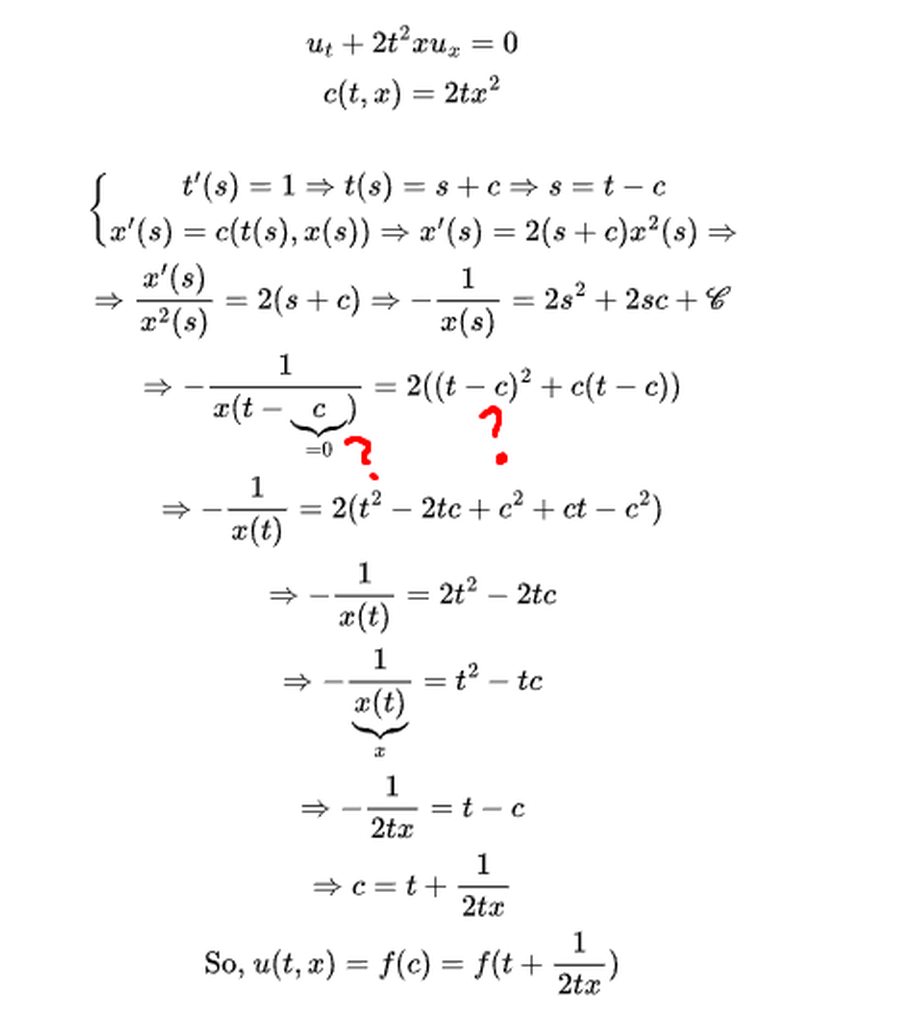[lilac barn]

It's a typo I would think as they later onwards just identify x(t) by x.

[lone goblet]

I think that might be it

[lone goblet]

I have another question regarding this other solution.
Where did 1/z(0) come from in that solution to the differential equation?
Looks like they just took the constant from the solution of the antiderivative and made it equal to 1/z(0) or something. But why?

[lilac barn]

The boundary condition from integrating the left side. Also for such question, use #odes-and-pdes

[lone goblet]

what do you mean by "the boundary condition"?

[maiden spindle]

How do I come up with a Lyapunov function for f(x,y)=(2y^3 - x^5, -x-y^3+y^5)? I'm getting really lost. Is there a standard way of finding one? I think that the critical point (0, 0) of the ODE (x', y')=f(x,y) is asymptotically stable since numerical solutions plotted near that critical point converge to it.

I tried expressing g(x,y)=L_{f(x,y)} Q (directional derivative of Q:R^2 -> R in the direction of f(x,y) at (x,y)), and then computing the derivative of g to try and find Q such that g is negative definite in a neighborhood of (0, 0), but I am getting nowhere.

[acoustic minnow]

You're integrating over s from 0 to s

[misty needle]

How did you learn the finite element program for magnetohydrodynamic equations

[buoyant pike]

Please don't post your question in multiple channels

[misty needle]

okey

[hallow pumice]

yoo damn

[lone goblet]

Is my solution to this PDE problem correct? https://imgur.com/a/98Lh0XP

I really am not sure if my approach is correct or not and I would appreciate if someone would help me find if my solution is valid or not.

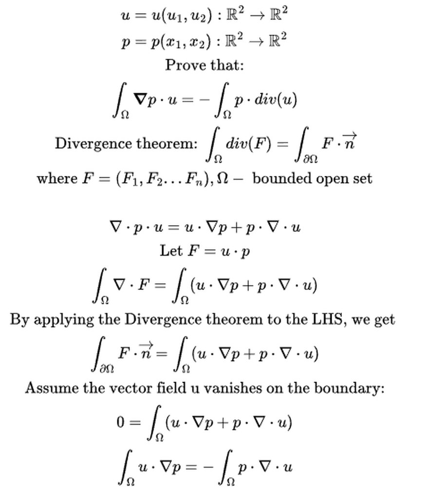[spare sentinel]

Question regarding fractional sobolev spaces defined through FT and distributions, I would like to formally understand the following definition

$W^{s,p} = { u \in \mathcal{S}^\prime , \vert , \mathcal{F}^{-1}((1+{\vert \xi \vert}^2)^{s/2}\mathcal{F}(u)) \in L^p}$

I don't understand how $(1+{\vert \xi \vert}^2)^{s/2}\mathcal{F}(u)$ is meant, if it meant as a distribution thus as

$\mathcal{F}(u)((1+{\vert \xi \vert}^2)^{s/2} \cdot \varphi)$

It doesn't work cause $(1+{\vert \xi \vert}^2)^{s/2}$ isn't smooth enough. The only way to understand it from my perspective is, if we assume, that $\mathcal{F}(u)$ is an integrable function for some p or that $\mathcal{F}(u)$ is measurable and it defines with the mutplier a solid distribution. So how is this definiton meant to be read?

[untold delta]

KIl

[spare sentinel]

shouldn't the p be mapping to $\mathbb{R}$ instead of $\mathbb{R}^2$? If so then it look alright if you have the correct differentiability assumptions on u and p

[untold delta]

KIl

[brave bay]

What do you mean when you say that $(1+|\xi|^2)^{s/2}$ is not smooth enough? Isn't it $\mathcal{C}^\infty$?

[untold delta]

4453

[spare sentinel]

ok fuck me

i take this as a big F

thank you i was far to focused on the s/2

[brave bay]

Don't worry about it, it happens.

[lone goblet]

yes you are right it is mapping to $\mathbb{R}$

[untold delta]

xbr

[astral vine]

In fact Bessel potential of any order s preserves the Schwartz class and is continuous w.r.t to the topology on the space made of Schwartz functions. In particular by duality it preserves continuously the class tempered distributions.

Thus this ask you if for a tempered distribution f, you can represent the tempered distribution (I-∆)^s/2 f by a Lp function

(Representation theorem for duality of Lp spaces)

[spare sentinel]

Ok then another question maybe you know this, the fractional sobolev space (via Gagliado-SemiNorm) or the bessel space (through Bessel potential), for both of these spaces when do I know that the fractional Lalplace is defined (mutplierer with |xi|^s in FT) besides the case where p = 2?

[lilac barn]

I think usually you just check if the multiplier is bounded in Lp (defined on a dense subspace with bounded extension) and for that a sufficient condition is the Mihlin-Hormander multiplier theorem.

[astral vine]

Exactly what Coat said

But for Bessel potential spaces you define it through the tempered distribution stuff

Then you can work with the formulation to show that, when s is non negative, your tempered distribution, whose image under the Bessel potential is represented by an Lp function, is then also an Lp function itself.

[spare sentinel]

Ok great but no general statement known for it?

[astral vine]

There is

Check Hao's lecture notes on harmonic analysis.

[spare sentinel]

ah hell yeah thanks thats the kind of definitions i wanted thank you so much

its so much chaos if you try to get some info about fractional sobolev and laplacian without much headaches

[maiden spindle]

Is there a Lyapunov function for the critical point $(0,0)$ of $\dot{x}=2y^3-x^5$, $\dot{y}=-x-y^3+y^5$?

[untold delta]

Beous

[maiden spindle]

Cause numerical solutions make it look like it's asymptotically stable.

but this thing feels impossible to find

[tired hollow]

Still have to write a conclusion, add equation numbers, and clean some stuff up like grammar and punctuation

Please tear me a new one

I think my section on method of characteristics is a bit lacking I dont have time to go deeply into the concept

and add a bibliography

[fringe onyx]

Maybe im tripping but isnt this false? Feels like we need a uniform bound on the measure of the complement of suppu here. If it is in fact true please don't give me any hints since this is a assignment

Just want to make sure there isnt a mistake

[astral vine]

This heavily true and a fudnamental result in pde theory, geometry, spectral theory, and many other realted subfields

[fringe onyx]

okay ill get back to it then

thanks

[astral vine]

All the assumptions are really important there

they all matter

[fringe onyx]

Okay i figured it out

the issue was that i was trying to relate things to the version we had seen in class (|u-u_Omega| instead of u) which cant even work if the domain isnt Lipschitz anyways, and even if it was I could only figure stuff out that needed uniform bounds as mentioned above

but turns out it's just a simple IBP+Holder

[astral vine]

This one is Poincaré(-Sobolev)-Wirtinger inequality

The one you have shown before is the Poincaré(-Sobolev) inequality

[lilac barn]

A thing to note is that the main counterexample are the constants. Both try to just weed this counterexample out: either by requiring mean 0 or requiring vanishing at boundary

[fringe onyx]

yeah the moral of it is clear to me

thanks a bunch

[minor mulch]

in fact the minimal constant C reflects some aspect of the geometry of the domain Omega.

more precisely, it is intimately related to questions of isoperimetry.

[misty needle]

Why does proving this indicate that the format is stable

[lilac barn]

What is their definition of unconditional stability?