#numerical-analysis
1 messages · Page 10 of 1
 solid igloo
I mean, should I pay close attention to the different topologies that happen in rudin's functional analysis? Or should I focus on normed spaces or Banach spaces, to assume almost all theorems hold, without having to remember so many topologies.
Each of his theorems have different hypotheses that make it much difficult to track. Maybe I just have to study harder and it will be worth it? I heard there is even functional analysis on graphs that would be cool
 sinful idol
solid igloo
I mean, should I pay close attention to the different topologies that happen in ...
sinful idol
solid igloo
I mean, should I pay close attention to the different topologies that happen in ...
Sobolev spaces
 pine jettyBOT
Evil Bean


 delicate falcon
yo
 heady mesa
 wary scarab
The one on the left probably won't converge.
Whereas the one on the right does.
$ln(1)=0$ so $\frac{1}{\ln(x)}$ is going to have a vertical asymptote in this domain.
Why is this important?
At an asymptote the derivative is going to be massive and is going to get bigger.
(I'd suggest actually differentiating and observing the derivative of the function on the right in this domain).
Whereas the expression on the right has a nice derivative and is a smooth function on the domain.
I'd suggest looking up the 1D Fixed point theorem, one of the conditions is that near the root you need: the function to have an absolute derivative less than 1.
pine jettyBOT
Max

 idle cosmos
Hello, I have a question about the rayleigh quotient itération. Whats the theorical convergence of the method if x0 (the initial vector we choose) and v (the eigenvector to wich we converge) if |x0-v| > 1 ?
 wide spear
Have you looked at the convergence proof in Demmel
 kind copper
wide spear
Have you looked at the convergence proof in Demmel
kind copper
wide spear
Have you looked at the convergence proof in Demmel
Nah but I can ask him he’s my professor rn 😭
kind copper
Yeah lmao how you know
wide spear
I too took 221 with jim
kind copper
LMAO
wide spear
Anyways you should read the proof in the book before asking him
 unborn cedar
i had this qn i had to answr
Let ℝd be equipped with the Euclidean norm, let D⊂ℝd be a closed set, let g: D→D be a contraction with Lipschitz constant L=1/3, let x0∈D and assume that D⊂B2(x0). By the contraction mapping principle, there exists a fixed point x*∈D of g, and the sequence (xk)k generated by the iteration
x_{k+1}=g(x_k)\quad\text{for}\ k\in\mathbb{N}
converges to x*.
What is the smallest number N∈ℕ such that for any dimension d≥1, and for any D, g and x0 as characterised above, we have
x_k\in B_{10^{-8}}(x^*)\quad\forall,k\ge N?
Hint: Consider the concrete example D=[0,2], g(x)=x/3 and x_0=2 and find the index N_1 in that particular case; this shows that, in general, the smallest possible N working for all cases is larger N_1.
To then find an N that works for all cases of D,g as in the statement of the question, you have to write down a short mathematical argument. You manage to make N=N_1, you have identified N.
the answer is N=18
ok nice the latex didnt convert

this is the written explanation for why n=18 but tbh i dont really understand lol...like the whole shabang. if anyone could help me out id be forever grateful 🙏

 edgy zinc
What does "$O(1)$ numbers" mean?
My understanding is that if $f=O(g)$, then there exists $C>0$ s.t. $\qty| \frac{f(x)}{g(x)} | \leq C$
So if you say a constant $A$ is $O(1)$, you're saying that $|A/1|=|A|\leq C$, which doesn't seem to be particularly meaningful, as it is true of every number

 pine jettyBOT
Douglas
 edgy zinc
wide spear
Order of magnitude
edgy zinc
wide spear
Order of magnitude
Meaning what exactly?
edgy zinc
okie dokie
wide spear
unborn cedar
this is the written explanation for why n=18 but tbh i dont really understand lo...
Which part don’t you understand?
edgy zinc
wide spear
A and B are close to 1
related question... given that A=O(1) means A is close to 1, I presume it means that A=[integral up to some point in the interval]/[integral over entire interval], rather than just the numerator?

cos if the total integral is 4π eg and A is just the integral across some fraction of the interval, then A might be 11 or something, in which case A is certainly closer to 10 than 1
edgy zinc
edgy zinc
related question... given that A=O(1) means A is close to 1, I presume it means ...
this is in the context of the trapezium rule btw
wide spear
Scaling an integrand by a constant doesn't change any of the theory
edgy zinc
wide spear
Scaling an integrand by a constant doesn't change any of the theory
what's the significance of specifying O(1) then, as opposed to O(10), or any other?
 molten knot
edgy zinc
what's the significance of specifying O(1) then, as opposed to O(10), or any oth...
molten knot
edgy zinc
what's the significance of specifying O(1) then, as opposed to O(10), or any oth...
f=O(1) means f<=C*1 for some c>0
O(•) implicitly means some constant times the general order of convergence
so we pull out all constant terms into that C
wide spear
edgy zinc
what's the significance of specifying O(1) then, as opposed to O(10), or any oth...
Machine epsilon is the distance between 1 and the next floating point number
edgy zinc
wide spear
Machine epsilon is the distance between 1 and the next floating point number
right but what does eps have to do with O(1)?
wide spear
eps changes when you get further away from 1
 barren brook
does anyone know how we can compute an error bound for Romberg integration?
wide spear
Start with the error bound for the trapezoidal rule, then see how the error behaves under Richardson extrapolation
barren brook
wide spear
Start with the error bound for the trapezoidal rule, then see how the error beha...
Thank you. I will try that
edgy zinc
How are we getting 5.27?

 wide spear
What is S_i defined as
edgy zinc
wide spear
What is S_i defined as
It's defined as in 5.21


 brave crypt
When doing quadrature by decomposing domain into piecewise polynomial approximations(lagrange), is there anything we can say about the error depending where you are at in the interval?
To restate:
For lagrange polynomial interpolation the error increases at the bounds. What can we say when we do a piecewise polynomial interpolation? What about in case of quadrature?
wide spear
Do you mean that the error is large at the endpoints of the interval?
brave crypt
Yea not bounds
wide spear
This is dependent a lot on grid spacing
brave crypt
Well assuming equidistant
wide spear
For the interpolation points used for the polynomial approximation
Ok well equidistant points are bad
brave crypt
Yes but it doesnt matter for quadrature
wide spear
For quadrature, you can do better with non equidistant points
At any rate, this is the error for polynomial interpolation

For interpolation points x_i
The product on the right hand side will vary in your interval, and for equidistant points, is minimized at x=x_i and x at the center of the interval
brave crypt
Yea I get this but I guess my question was more about quadrature because it was covered in class recently
We discussed newton cotes formulas
And we also discussed a possible way to minimize errors was by breaking the integration interval into subintervals and applying polynomial interpolations there
brave crypt
wide spear
Yes newton cotes is unstable for high degree unless you are very careful
Yea we talked about that a little. I don’t know the extended story though.
I guess my question was more like can we say anything about where error is highest or lowest when doing this subinterval polynomial interpolation
As it relates to quadrature tho
wide spear
brave crypt
Yea we talked about that a little. I don’t know the extended story though.
Well, precisely because equidistant point based polynomial interpolation is useless at high degree
wide spear
You don't want your interpolation weights to come from a polynomial interpolation
You want to do a least squares method to get the weights instead
 hasty ferry
How can one show: A matrix ( A \in M_n(\mathbb{R}) ) is invertible if and only if there exists a permutation matrix ( P \in \prod_n ) such that all principal minors ( (P \cdot A)_m ) of ( P \cdot A ) are invertible for ( m = 1, \dots, n ).
pine jettyBOT
Sentinel
 wide spear
Hmmm #linear-algebra
hasty ferry
its actaully from a numerical analysis lecture
thats why i posted it here
but it may not fit here u are righjt
hasty ferry
wide spear
I understand but there is a linear algebra fact
would you like to help 🙂
wide spear
I regret to inform you that I do not want to think about permutation matrices at the moment
hasty ferry
wide spear
I regret to inform you that I do not want to think about permutation matrices at...
Thanks though i ve posted it in linear algebra with my intended solution
which doesnt work fully
brave crypt
I dont know either but my guess is something like invertible principle minors things relates to gaussian elimination way of finding determinants
And you want to show thats non zero
Id try that atleast
 wicked pecan
wide spear
Yes newton cotes is unstable for high degree unless you are very careful
wicked pecan
wide spear
Yes newton cotes is unstable for high degree unless you are very careful
Yeah isn’t that cus of evenly spaced points?
Just staying I read none of the messages above or below that message I just saw it and instantly replied
wide spear

 orchid lagoon
I have a question about subspace iteration. If we run this algorithm on symmetrical matrices to calculate the 10 largest eigenvalues. We simulate matrices with size ranging from 10 to n. I simulated my algorithm and for each bigger matrix n, I saved the amount of iterations until convergence.
The relation between amount of runs & size of matrix was linear. But I fail to understand why...
wide spear
By subspace iteration, do you mean arnoldi iteration?
orchid lagoon
I'm not sure what arnoldi iteration is. I use this algorithm:

Iteration matrix Q, QR decomposition in second step
I really appreciate your reply
 raven panther
Hey
im trying to read more about butcher tablaues, implicit RK and diagonally implicit RK methods, where do i look at?
my ultimate goal is implementing a parallel DIRK solve
raven panther
wide spear
Like resources?
Yes
im pretty much vanilla in numerical analysis
just learned about runge-kutta a couple of days back
wide spear
This should be good
I'm not entirely sure what you mean by a parallel DIRK solve
Like do you have a pde that you want to use DIRK to time step for
Or are you trying to do a parallel in time thing
raven panther
yk normal parallel RK?
parallel in time yes
you can set it up for implicit and diagonally implicit RK as well
wide spear
orchid lagoon
If I have a sparse matrix and I assign it as sparse(B) in matlab. Then when doing gram schmidt on vectors, do I have to do this step? vector1 = sparse(vector1 ./ norm(vector1));
Mister angetenar, does this statement ring any bells?
Hmmm, operations in gram schmidt might make elements nearly zero instead of zero, which would make a vector not sparse anymore
hmmmmmmmmm
wide spear
Gram Schmidt is generally not preferred for a numerical algorithm
Are you doing a QR factorization?
orchid lagoon
Yessir, and Gram Schmidt is obligatory
wide spear
What do you mean obligatory
orchid lagoon
EUh if I don't do it I won't pass
wide spear
Ok
orchid lagoon
Is it correct that that algorithm can cause 0 elements to become non zero?
wide spear
orchid lagoon
Hmmm, operations in gram schmidt might make elements nearly zero **instead of ze...
Gram schmidt will not preserve sparsity
Check the modified gram-schmidt presented here
orchid lagoon
So my matrix becomes non sparse, but would zero elements become non zero?
ok I will check it out, thanks angetenar!
edgy zinc
Why are the nodes indexed by n,i rather than i only?
 edgy zinc
So when he refers to "two groups of parameters", they are the nodes and the approximation weights, not n and i?
wide spear
The author may be trying to emphasize that the x_n,i will vary with different numbers of quadrature points
wide spear
edgy zinc
So when he refers to "two groups of parameters", they are the nodes and the appr...
Paramters isn't the best term, I would say degrees of freedom
But yes, you can vary the qudrature nodes and the quadrature weights at each node
edgy zinc
right ok
 fathom rain
edgy zinc
Why are the nodes indexed by n,i rather than i only?
fathom rain
edgy zinc
Why are the nodes indexed by n,i rather than i only?
I would say it is more common to use x_{i,n} but it just means x_{n,i}=h*i+a=(b-a)i/n+a, i=0...n
(or some other grid)
fathom rain
edgy zinc
just wondering wot was up with the notation
for a specific grid type, the node points are usually defined by n and the point indices i, not more complicated
and if you use multiple grid types you need one or more extra indices to define which
edgy zinc
I am not seeing the thing that is supposed to be easy to see (5.48)


 wide spear
Have you done the integration by parts k+1 times
edgy zinc
wide spear
Have you done the integration by parts k+1 times
This is as far as I got before thinking I had gone wrong somewhere

there should be alternating signs in the margin of the D/I table
wide spear
You can ignore the n!/(2n)!, that won't affect the integral
edgy zinc
yeah i included the n! (and not the (2n)!) so as to avoid a 1/facotrial thing
wide spear
Hmmmm
edgy zinc
edgy zinc
yeah i included the n! (and not the (2n)!) so as to avoid a 1/facotrial thing
it just makes the table look a little bit tidier i think
wide spear
Yeah sure
Ok let's see how I would do this
First, recognize that if n is even, then phi_n only contains even degree terms
Similarly if n is odd, then phi_n contains only odd degree terms
So if n is even and k is odd or vice versa, the integral will be 0 right
Integral of an odd function on a symmetric interval
wide spear
Now, we consider when both n and k are even
Hmmmmm
Ok really what you should do is show that the integral of phi_n(x) from -1 to 1 is 0
There are much better presentations of Legendre polynomials that actually discuss their properties
(Namely being an orthogonal basis)
(In which case 5.48 follows immediately)
edgy zinc
wide spear
(Namely being an orthogonal basis)
how exactly does this argument work in this context?
we have an inner product $(f,g)=\int_{-1} ^1 f(x) g(x) \dd{x}$
then what?
pine jettyBOT
Douglas
 edgy zinc
(phi_i, phi_j)=0, i≠j, is what we're saying?
wide spear
Yes
edgy zinc
and how does that get you (x^k, phi_n)=0
wide spear
If k<n, then you can write x^k as a sum of phi_i for i<=k and split the integral up
And each piece of the integral will be 0
edgy zinc
hmmmm yes
you are right this is a much nicer argument than doing the integral by tabulation
ty for the help
wide spear
<@&268886789983436800>
 unkempt moth
gone
 bold marsh
Anyone here knows about b-spline?
 grave spoke
What about it?
bold marsh
grave spoke
What about it?
I just want to understand it, for example what are the knots and control points in a spline?

Also how do I define a B-spline?
grave spoke
bold marsh
I just want to understand it, for example what are the knots and control points ...
Sorry, I'm a bit preoccupied rn, but I can try to answer later if no one does
bold marsh
grave spoke
Sorry, I'm a bit preoccupied rn, but I can try to answer later if no one does
np, tysm
 alpine mirage
bold marsh
I just want to understand it, for example what are the knots and control points ...
alpine mirage
bold marsh
I just want to understand it, for example what are the knots and control points ...
so basically you first choose some arbitrary knots, which are points on the x-axis
this choice defines a set of functions constructed with a recursive relation, where each function (B-spline) is nonzero only on some limited interval
and then you choose control points, which are something like coefficients in linear combination of vectors
but in multiple dimensions
so you take some average of these B-splines (basis splines) weighted by control points
or if you're familiar with the notion of partition of unity, it's a very similar idea with basis splines as functions
bold marsh
What is this term? I looked it up and it says blending functions that are used to blend the control points
 alpine mirage
yea, maybe it's better to view it as a weighted average of control points
B-splines look something like this

if you enforce them to sum up to 1, you get something like a "smoothly changing weight" for the weighted average of control points
alpine mirage
alpine mirage
or if you're familiar with the notion of partition of unity, it's a very similar...
yea exactly
bold marsh
alpine mirage
yea exactly
Another question, how do I calculate the points on the b-spline curve?
I read that there's an Algorithm called DeBoor-Cox
But how to apply that Algorithm?
I found the Cox-de boor formula
bold marsh
alpine mirage
yea exactly
tysm, for explaining b-spline
alpine mirage
bold marsh
Another question, how do I calculate the points on the b-spline curve?
sorry i had a call
yeah you apply the Cox-de boor formula which is just computing the values recursively from the splines of lower degree
bold marsh
I forgot to mention that I'm making a presentation about b-spline
 azure socket
bold marsh
I forgot to mention that I'm making a presentation about b-spline
azure socket
bold marsh
I forgot to mention that I'm making a presentation about b-spline
I have an amazing video for you to watch then

why are splines? well my god I have good news for you, here's why splines!
if you like my work, please consider supporting me 💖
https://www.patreon.com/acegikmo
This project grew much larger in scope than I had originally intended, and burnout made it impossible for me to do more with it. It was already getting incredibly unwieldy, so I apolog...
you caaan skip straight to the B-Splines chapter (also what I did originally) but you will likely end up watching the whole video. especially if youre presenting on b-splines, like I had to
shes really good at telling the story and the visuals just keep you entranced
wide spear
Care to copy over what is going on
 coarse root
wide spear
Care to copy over what is going on
coarse root
wide spear
Care to copy over what is going on
I'm using a modified Newton's method for solving a 2x2 non-linear system. I've substituted the Jacobian's elements with the following expressions:
[
\begin{cases}
\frac{\partial f_1}{\partial K_1}\approx\frac{f_1(K_1+s,,K_2)-f_1(K_1,,K_2)}{s}\
\frac{\partial f_1}{\partial K_2}\approx\frac{f_1(K_1,,K_2+s)-f_1(K_1,,K_2)}{s}\
\frac{\partial f_2}{\partial K_1}\approx\frac{f_2(K_1+s,,K_2)-f_2(K_1,,K_2)}{s}\
\frac{\partial f_2}{\partial K_2}\approx\frac{f_2(K_1,,K_2+s)-f_2(K_1,,K_2)}{s}
\end{cases}
]
wide spear
What system are you solving
pine jettyBOT
Eruc
 wide spear
Also what are you plotting
coarse root
The truncation error (Y) plotted against different values for the small supplement s in the expressions (X).
The truncation error is the total of the entire problem (it's a combination of different methods feeding into each other) but the only thing being varied here is the value of s
coarse root
wide spear
Or after it's converged?
After 6 iterations, sufficiently converged for the problem
But so it seems there's a certain value of s that minimises the truncation error, and then it grows, and then starts approaching the same minimum asymptotically. What's going on with that? Where can I look more into this?
wide spear
Hmmmm
It's hard to say what is going on without knowing more about what f is, but this kind of reminds me of what happens when you vary the parameter in successive over relaxation
coarse root
wide spear
What system are you solving
To be more specific, the system being solved is to optimise two constants of a second order non-linear ODE so that the solution to the ODE fullfils two separate criteria
So the entire problem involves errors from ODE-solving (RK4), polynomial interpolation, Newton-Rhapson, and then this error dependent on s
wide spear
Are the two lines two different error measures
coarse root
They're the errors of the two different constants being optimised
wide spear
pine jetty
**Eruc**
What does f look like
coarse root
I don't really have a expression for them, but f1 gives the distance between two points on the ODE curve that have two specific properties. The constants are being optimised so that f1 = 0 (i.e. the same point is supposed to have both properties)
And f2 is something similar but less complicated
wide spear
Do you have any method of directly computing the error in the derivative calculation of f
 violet gull
Hey guys, what's the link between the fourier transform and the fourier series? If there is one at all. I kinda what they each are on their own, not sure how they relate though. Thanks 🙂
wide spear
Fourier series are the Fourier transform on a periodic interval
Ask further questions in #advanced-analysis
 midnight plover
im using gauss seidel iteration (+ overrelaxation) to remove the divergence from a velocity field when simulation the incompressible uniform euler fluid equations, but its slow for high resolutions because i need a bunch of iterations. when iteratively reducing the divergence im subtracting it from the velocity field at every step.
i want to use a multigrid method but im confused on whether im supposed to be projecting and restricting the actual velocities of each cell (thus seemingly destroying local information when interpolating back onto the fine grid) or if im supposed to keep a separate error array, and after solving for it at each level interpolate it onto the fine grid by subtracting it from the actual velocity array (thus keeping local velocity differences but subtracting an interpolated divergence term)
midnight plover
like what
wide spear
Compatible finite elements or a Lagrangian approach a la Chorin's vortex method
sinful idol
Projection methods avoid having to deal with divergence too
edgy zinc
wouldn't it make more sense to use the notation $P_N (n)$?
N is a parameter that we control, whereas n is entirely random


 pine jettyBOT
Douglas
 edgy zinc
wide spear
I wouldn’t think too much about it
edgy zinc
wide spear
I wouldn’t think too much about it
maybe
but it feels weird
like you wouldnt diffeentiate wrt an index
i mean you could
but it would be a little weird
wide spear
Ratking behavior is not channel appropriate
edgy zinc
oh
wide spear
Rafiking
At any rate, there is far worse notation that you will come across I imagine
edgy zinc
Why is $\sigma$ not equal to $p_1 p_2/N$?
This is what you get if you compare coefficients of 5.67 and 5.68

 pine jettyBOT
Douglas
 wide spear
edgy zinc
wide spear
edgy zinc
ye sorry these are from my numerical methods lecture notes
so just defaulted to this channel
but u r correct
prob makes more sense here
kind copper
Does anyone know why for sparse matrices randomized truncated SVD (like Halko et al.) performs empirically poorly something like Arnoldi iteration (for example ARPACK)? Specifically for PCA
brave crypt
In my numerical analysis course. We get some theory questions too. Like what are the draw backs of newton ralphson theory. The topics we have are.
- Error calculation
- taylor theorem
- Newton raphson method
- secant method
- bisection method
- interpolation (linear quadratic)
- newton dividend diff interpolation
- lagrangian
- trapeziod
- Simpsons 1/3 rule
How do i study the theories. I never studied theory for maths before and our teacher does not tell us
Can ppl here tell me?
 normal mauve
Anyone has good recommendations for introductory books on numerical optimisation?
 vapid plume
brave crypt
In my numerical analysis course. We get some theory questions too. Like what are...
vapid plume
brave crypt
In my numerical analysis course. We get some theory questions too. Like what are...
I would say just read books, there are many good books on numerical methods/analysis. I recommend James F. Epperson's book, it is very good at the introductory level. You can always search on the web for other recommendations or ask in the books channel.
brave crypt
okay thank you very much ❤️
sinful idol
brave crypt
In my numerical analysis course. We get some theory questions too. Like what are...
A good classic is "An Introduction to Numerical Analysis" by Atkinson.
sinful idol
normal mauve
Anyone has good recommendations for introductory books on numerical optimisation...
Nocedal should be the one of the most commonly used.
brave crypt
can i send link here?
we are following a book at uni and that book is uploaded in internet by the ppl i think
Numerical Methods with Applications by Authors: Autar K Kaw | Co-Author: Egwu E Kalu, Duc Nguyen
sinful idol
normal mauve
Anyone has good recommendations for introductory books on numerical optimisation...
You can also check out convex optimization books, usually they include a significant amount of numerical algorithms inside.
brave crypt
normal mauve
Anyone has good recommendations for introductory books on numerical optimisation...
https://nm.mathforcollege.com/textbook-numerical-methods-with-applications/
chapter 9 is optimization
sinful idol
brave crypt
Numerical Methods with Applications by Authors: Autar K Kaw | Co-Author: Egwu E ...
Sounds like a very applied book.
brave crypt
sinful idol
Sounds like a very applied book.
ikr but we get question in exam like:
- in which of the following function does root jumping occure while useing the newton raphson methods? analyse graphically.
a. y = x^2
b. y = sinx
c. y = cosx
this is maybe explanation of the draw back of newton.
idk
sinful idol
brave crypt
ikr but we get question in exam like:
1. in which of the following function does...
Um... this is an applied question.
sinful idol
The maths i know is proof based maths
wide spear
What is wrong with that question
sinful idol
Nothing wrong, but its something where you can just draw and guess.
No proof needed.
But not a theoretical question (in my opinion).
 minor osprey
It seems fine as introductory if you aren’t really coming from a math background. Seems like the book is geared towards engineering majors
 real hull
hello, does anyone have any references for error analysis/estimation for various spline interpolation methods? (cubic spline, spline with tension, thin plate spline), or does anyone know any methods and can explain?
wide spear
Taylor series
sinful idol
real hull
hello, does anyone have any references for error analysis/estimation for various...
Most approximation theory textbooks should cover rigorous error estimates for splines.
The techniques used depend on the function spaces. For instance, taylor series would work for C^k functions but probably not so helpful for H^k functions.
 woeful schooner
Hello everyone i need a reference for the research im doing on weddle’s method so if anyone could help me i would appreciate it alot
fathom rain
woeful schooner
Hello everyone i need a reference for the research im doing on weddle’s method s...
Seems to be an obscure Newton-Cotes method, never heard of it 🙂
so I assume compare it with with the standard ones?
fathom rain
woeful schooner
Hello everyone i need a reference for the research im doing on weddle’s method s...
 marble socket
I want to choose $n+1$ pairwise distinct points $x_0, \dots, x_n \in [0,1]$ to extremize the value of the integral
$$L = \int_0^1 |w(x)| , dx, \qquad w(x) = \prod_{k=0}^n (x - x_k).$$
I know that $L$ is minimized when we take the $x_k$ to be the zeros of the Chebyshev polynomial of the second kind $U_{n+1}(x)$. But what choice of the $x_k$ maximizes $L$?
pine jettyBOT
Eduardo León
 wide spear
Lol
 teal panther
LR = A where L and R are up and down triangle matrizes, prove that $\frac{|| \left|L\right|\left|R\right| ||\infty}{||A||\infty} \leq \kappa_\infty(L)$
pine jettyBOT
Jemaseda
 teal panther
can someone help me with this? i have no idea what im doing
wide spear
What have you tried
teal panther
wide spear
What have you tried
Well not much pure algebra playing and the < things to approximate or smtn
wide spear
Well you can prove it for diagonal matrices at least right
molten knot
any suggestions on how to handle (d)? I tried the hint but I keep getting cross terms that I dont know to handle

the derived scheme with $f=0$ is
$$\frac{1}{2}(W_2^{m+1}+W_2^{m},\chi)=\frac{1}{\tau}(W_1^{m+1}-W_1^{m},\chi)$$
$$a(\frac{1}{2}(W_{1}^{m+1}+W_{1}^{m}),\chi)=\frac{1}{\tau}(W_2^{m+1}-W_2^{m},\chi).$$
pine jettyBOT
ansh
 molten knot
W^(m+1/2)=(W^(m+1)+W^(m))/2 btw
wide spear
Well what do you get after multiplying the system
molten knot
wide spear
Well what do you get after multiplying the system
so if i test eq1 with $W_1^{m+1/2}$ and eq2 with $\triangle_h W_2^{m+1/2}$ the new system is
$$(W_1^{m+1/2},W_2^{m+1/2})=\frac{1}{2\tau}(|W_1^{m+1}|^2-|W_1^{m}|^2)$$
$$(\triangle W_1^{m+1/2}, \triangle W_2^{m+1/2})=-\frac{1}{2\tau}(|\nabla W_2^{m+1}|^2-|\nabla W_2^{m}|^2)$$
pine jettyBOT
ansh
 molten knot
(with some rearranging and integrating by parts)
but how do you show stability from here?
oh theres a typo it should be grad(W2) instead of grad(W1) in the second equation RHS
alpine mirage
is there some standard method of computing step in multivariate newton method up to quadratic term in taylor expansion
$$ 0 = f(x) + Df(x) h + \frac 1 2 D^2 f(x) (h, h) $$
how to get h is my question
pine jettyBOT
Bwoonoid, a crank
 wide spear
Newton's method for root finding?
I've literally never seen anyone include the quadratic term before lol
alpine mirage
wide spear
I've literally never seen anyone include the quadratic term before lol
the exercise probably aims to show that including it is not needed
theoretically it could make sense however, but idk how to calculate the step
edgy zinc
Where is A+B=1 coming from? Is that imposed just to make A and B "nice" numbers?
 wide spear
If you are integrating a constant function, you need A+B=1 for the quadrature to be correct
This is a common thing that you'll see in numerical quadrature
edgy zinc
wide spear
If you are integrating a constant function, you need A+B=1 for the quadrature to...
what's quadrature?
wide spear
Numerical integration
wide spear
You are integrating an arbitrary function f yes
edgy zinc
so how does
If you are integrating a constant function, you need A+B=1 for the quadrature to be correct
help us with integrating arbitrary f?
wide spear
It's a basic check on accuracy for the easiest functions to integrate
If you cannot numerically integrate a constant, then you have no hope of doing anything more sophisticated
 tall cypress
Hi guys, can I get some help? Suppose $$A = \begin{bmatrix} A_{11} & A_{21}^T \ A_{21} & A_{22}\end{bmatrix}$$ is symmetric PD. I want to prove that $|A_{21}A_{11}^{-1}|2 \leq \kappa{2}(A)^{1/2}$, where $\kappa_2$ is the condition number under the operator 2-norm. The hint is considering $A$'s Cholesky factorization, but I can't seem to figure it out...
pine jettyBOT
{Wilhelm}
 wide spear
Well, what is the cholesky factorization of A
tall cypress
We don't assume anything about its factorization, only since it is PSD it can be done. The hint suggests using the block Cholesky factorization $$A = \begin{bmatrix}R_{11}^T & 0 \ R_{12}^T & R_{22}^T \end{bmatrix} \begin{bmatrix}R_{11} & R_{12} \ 0 & R_{22}\end{bmatrix}$$
pine jettyBOT
{Wilhelm}
 tall cypress
Where $A_{11} = R_{11}^TR_{11}$ is its Cholesky factorization itself
pine jettyBOT
{Wilhelm}
 tall cypress
I managed to bound it by $\kappa_2(A)$, but not its square root
pine jettyBOT
{Wilhelm}
 tall cypress
I really appreciate any insights :)
tall cypress
2 norm
This is part (c) of an exercise, and this is what I have proved so far, first this factorization: $$\begin{bmatrix} I & 0 \ -A_{21} A_{11}^{-1} & I \end{bmatrix} \begin{bmatrix}
A_{11} & A_{21}^\tp \ A_{21} & A_{22} \end{bmatrix} \begin{bmatrix} I & -
A_{11}^{-1}A_{21}^\tp \ 0 & I \end{bmatrix} = \begin{bmatrix} A_{11} & 0 \ 0 & S
\end{bmatrix}.$$
pine jettyBOT
{Wilhelm}
Compile Error! Click the  reaction for more information.
(You may edit your message to recompile.)
 tall cypress
$\lVert A_{ij} \rVert_2 \le \lVert A \rVert_2, \quad i,j \in {1,2}$
pine jettyBOT
{Wilhelm}
 tall cypress
and $\kappa_2(S) \le \kappa_2(A)$
pine jettyBOT
{Wilhelm}
 tall cypress
Interestingly, the Schur complement $S$ simplifies to $R_{22}^TR_{22}$, and of course it should be enough to show that $|A_{21}A_{11}^{-1}|_2^2 \leq \kappa_2(S)$, which might be where the exercise is leading to
pine jettyBOT
{Wilhelm}
 tall cypress
Oh, I think the root part comes in by the fact that $\kappa_2(A) = \kappa_2(R^TR) = \kappa_2^2(R)$
pine jettyBOT
{Wilhelm}
 tall cypress
OHHHHH SOLVED IT :)))))
tall cypress
you use cholesky to show $A_{21}A_{11}^{-1} = R_{12}^TR_{11}^{-T}$, then the whole norm is less than $|R_{12}|2|R{11}^{-1}|_2$, and then you use the bound on block matrix norms above
pine jettyBOT
{Wilhelm}
 tall cypress
Ok, if anyone can give me a hint on this following problem that would be great:
Suppose that you have a solution to the following least squares problem,
$$
\min \left| \begin{bmatrix} A \ \textbf{c}^T \end{bmatrix} \textbf{x} - \begin{bmatrix} \textbf{b} \ d \end{bmatrix} \right|_2
$$
You can make no assumptions on the method that was used to solve it. How can you leverage the solution above to efficiently solve $\min |A\textbf{x} - \textbf{b}|_2$? The method should probably include the use of the Sherman-Morrison formula https://en.wikipedia.org/wiki/Sherman–Morrison_formula. Thanks!
pine jettyBOT
{Wilhelm}

 violet nymph
yo i think i desparately need some help
on numerical analysis
https://ustspace.s3-ap-southeast-1.amazonaws.com/upload/lbTzVGpf53mxcwyg286fCz60MufPq36f/FinalExam2019.pdf
I need some help with Q2, Q4 and Q5b
fathom rain
we wait 120mins and answer 😄
violet nymph
wide spear
You are practicing from a past exam?
yes
correct
this is a pastpaper from 2019

My progress so far with Q2
wait no the linear system is solved wrong
well to be honest now i am not too sure if my previous step is even correct
i somehow got a = (h-1)/(h+1) c
pls help
violet nymph
fathom rain
we wait 120mins and answer 😄
well that works too but this is a pastpaper lol
the year is written
 violet nymph
My current progress with Q4

But somehow the error term become zero
Idk what’s wrong for now, pls help
i will be back in around 3 hours, i need a quick nap
 barren star
I've recently started a project and I am trying to implement numerical methods using python.
https://github.com/TheKidKy/numerical_analysis

GitHub
numerical analysis methods using python. Contribute to TheKidKy/numerical_analysis development by creating an account on GitHub.
heady mesa
Nice, although I would suggest making sure you maximise the use of libraries if possible as they will use code, most likely written in C which is WAY faster than Python.
Python is generally considered slow, if you like the syntax but want more speed without losing the Syntax I'd recommend learning Julia
barren star
heady mesa
Python is generally considered slow, if you like the syntax but want more speed ...
should I switch to C?
heady mesa
Personally I would switch to Julia, but that has its own problems (slow compile times) but after that it is as fast as C but has a python feel
C is probably the fastest all around, ie. in compile time and run time
But python is the most convenient to code and there are lots of libraries
For instance, say you decide to use Python that would be fine just make sure to do as much code as possible in libraries such as Pandas, Numpy ext. which are written in C
Also Python has some really nice numerical analysis libraries such as Mpmath which I'm not sure the others have
violet nymph
hello guys i am back again

anyone have any idea on how to do Q5b?
FYI THIS IS NOT AN ONGOING EXAM, THIS IS A PASTPAPER FOR PRACTICE
violet nymph
violet nymph
yo i think i desparately need some help
on numerical analysis
https://ustspace.s...
to confirm this is not an ongoing exam, i am trying to do it since yesterday so....
wide spear
What have you tried
violet nymph
wide spear
What have you tried
well fun fact, i just found the proof in a textbook
wide spear
Lol nice
molten knot
violet nymph
taylor series expansion y around a and compute the difference
 neon remnant
hi
wide spear
Hello
 lofty widget
suggest any playlist for this topic man ..i have exams coming in 3months
heady mesa
Look at your notes and watch videos by topic rather than one set course...
this is the stage of maths where you need to be learning how to learn from notes and text as opposed to videos... as rarely does specialized content have video tutorials
 flat plank


This is how i decided to solve this.
As i'm supposed to pick 3 random ODE methods and either secant/bisection method for task b i have 6 possible solutions.
import numpy as np
from solvers import solver

# RHS of ODE
def rhs(t, y, m, k, g):
    v = y[1]
    dydt = v
    dvdt = -k/m * v**2 - g/m
    return np.array([dydt, dvdt])

def nonlinear_function(H, m, k, g, T, target_position, method):
    initial_conditions = np.array([0.0, H])

    # Wrapper
    def rhs_with_params(t, y):
        return rhs(t, y, m, k, g)

    t0 = 0.0
    dt = 0.01
    t, y = solver(rhs_with_params, initial_conditions, t0, dt, T, method)

    # Final position at t = T
    final_position = y[-1][0]

    # Return the difference from the target position
    return final_position - target_position

# Parameters
m = 1.3
g = 9.81
k = 0.05
T = 1.5
target_position = 10.0

# Differential methods
methods = ["Heun", "Ralston", "Runge-Kutta"]

# Results storage
results = []

for method in methods:
    print(f"\nUsing Differential Solver: {method}")

    def F(H):
        return nonlinear_function(H, m, k, g, T, target_position, method)

    # Bisection
    root_bisection = bisection(F, 0, 20)
    print(f"Bisection root: {root_bisection}")
    results.append((method, "Bisection", root_bisection))

    # Secant
    root_secant = secant(F, 0, 20)
    print(f"Secant root: {root_secant}")
    results.append((method, "Secant", root_secant))

print("\nSummary of Results:")
for method, solver, root in results:
print(f"{method} with {solver}: Root = {root}")```bisection() and secant() come from a worksheet we used in a lab and they're known to work
heady mesa
Fairs but it's numerical analysis
If you think there is a simple mistake it could be worth asking an AI chat bot, they good at picking up on simple mistakes
wide spear
Well they also didn’t ask a question
heady mesa
If you are just asking if it's right then look at the accuracy of your answer, are they accurate? If not how can you make it more accurate
wide spear
At least not that I can see
heady mesa
wide spear
Well they also didn’t ask a question
True 😭😂
heady mesa
heady mesa
If you are just asking if it's right then look at the accuracy of your answer, a...
/ what could you change to make your answer more accurate, if it doesn't make it more accurate then it's likely you've made a mistake
If you can't spot the mistake after a bit of investigation then just redo the whole thing again lmao honestly has helped me spot so many mistakes in the past
wide spear
!da2a
 copper abyssBOT
No need to ask “Can I ask…?” or “Does anyone know about…?”—it’s faster for everyone if you just ask your question! See https://dontasktoask.com/
heady mesa
copper abyss
No need to ask “Can I ask…?” or “Does anyone know about…?”—it’s faster for every...
Such a mathematician thing to say lmao
 idle light
Dear all, I having trouble with the discontinuous Garlerkin method (DG). My question is the following , by applying the DG method could I deduce a upwind/downwind discretization scheme for my PDE (a PDE to the convection diffusion type) ?
 final sleet
Is it true that accuracy in floating point numbers cannot be accurately calculated for precise precision and accuracy: https://en.wikipedia.org/wiki/Floating-point_arithmetic

In computing, floating-point arithmetic (FP) is arithmetic on subsets of real numbers formed by a signed sequence of a fixed number of digits in some base, called a significand, scaled by an integer exponent of that base.
Numbers of this form are called floating-point numbers.: 3 : 10
For example, the number 2469/200 is a floating-point number ...
 still forum
Yes, you can't rely on floating point numbers to be exactly accurate, try doing $0.1+0.2$ in python or something. Even if you write doing 0.3 on a computer, its really being stored as a slightly different number close to 0.3
pine jettyBOT
jamiecjx
 still forum
Floating point numbers generally only satisfy the standard arithmetic operations up to a known error, so for example, given floating point numbers $x,y \in \bb{F}$, we have $x \oplus y = (x+y)(1+\delta)$ where $|\delta| < \frac{\eps_M}{2}$ and a $\eps_M$ is a constant
pine jettyBOT
jamiecjx
Compile Error! Click the reaction for more information.
(You may edit your message to recompile.)
 still forum
said constant is usually about 2 * 10^{-15} in double precision, so whilst you can't calculate precisely with floating point, you can rigorously bound computations (with things like interval arithmetic)
 versed bison
also a related topic https://en.wikipedia.org/wiki/Machine_epsilon
 dusky pivot
Can someone please suggest me a good book/resource to study Runge Kutta methods, very funadmentally and in great detail? Would be great if it also mentions any suggestions on programming the different models of RK, like RK 7, 8 or higher in Python.
But, primarily I want to understand the method, the derivation of the formula, and it's application in real life problems.
 signal fiber
Apparently the golden ratio pops out of nowhere when doing natural cubic spline interpolation! Basically knots (nodes) at phi^2k makes the interpolation neither converge nor diverge. Is this well-known?

 sterile holly
I'm also open to using another library for this task.
I solved my first numerical eigenvalue problems yesterday lol.
Can someone please suggest me a good
sterile holly
I was helped :)
edgy zinc
please would someone explain the highlighted bit?

Also...
- "The case mu=1 is called "1-sublinear convergence". Don't you identify the nature of the convergence by the order q (q-convergence), so wouldn't it make more sense to say "the case q=1"?
- Why does he talk about mu=0 when the inequality mu satisfies prohibits that case? And what does it mean to lie between q=1 and q>1?

 vagrant jackal
if the approximation is correct to two decimal places then the errror (x_k - x*) is on the order of 10^(-3) meaning -log(x_k - x*) is somewhere between 2 and 3. similarly if they agree at 5 decimal places the expression would be 5--6
edgy zinc
vagrant jackal
if the approximation is correct to two decimal places then the errror (x_k - x*)...
ok
edgy zinc
edgy zinc
Also...
1. "The case mu=1 is called "1-sublinear convergence". Don't you identif...
what about this
vagrant jackal
edgy zinc
Also...
1. "The case mu=1 is called "1-sublinear convergence". Don't you identif...
if you say q = 1 then people would assume you are referring to the linear case unless otherwise specified. both special cases start with "1-" to refer to the order q
 obtuse vault
signal fiber
Apparently the golden ratio pops out of nowhere when doing natural cubic spline ...
obtuse vault
signal fiber
Apparently the golden ratio pops out of nowhere when doing natural cubic spline ...
Maybe you should look into why that is
That’s the beauty of math after all
edgy zinc
vagrant jackal
if you say q = 1 then people would assume you are referring to the linear case u...
so is it the case that if q=1 then 0≤mu≤1 (i.e. closed interval, not open)?
possibly one for probability, but what does it mean to choose the nodes?
the nodes are the data points, i.e. a random sample from a population, so how is there any choice in their spacing?
 wide spear
There are a few variants of the interpolation problem
One is scattered data interpolation where you have no choice over where the data is located
But in other cases, you might have a function that is very expensive to compute so you fit a polynomial approximation to evaluate it more efficiently
In which case you do have a choice over the interpolation nodes
 ionic veldt
Maybe someone here can help me with a question about numerical integration.
Specifically, the remainder theorem for the "midpoint method". I highlighted it in red.
I can't find a proof of this theorem anywhere that does not assume the second derivative of the function is continuous. The theorem's formulation seems to state only that the second derivative must exist, i.e., continuity is not guaranteed.
I have found only these proofs so far:
https://math.stackexchange.com/a/4327333/861268
https://www.macmillanlearning.com/studentresources/highschool/mathematics/rogawskiapet2e/additional_proofs/error_bounds_proof_for_numerical_integration.pdf
But they both assume continuity of second derivative.
I'm exhausted from searching. It feels like this is some completely unimportant detail.
P.S.: Maybe I should've posted it in calculus chat because I've found this theorem in calculus book? Here: https://openstax.org/books/calculus-volume-2/pages/3-6-numerical-integration
 heady mesa
Essentially you are approximating the curve using a straight line
Or in other words the first order Taylor series of the function.
Then integrating the straight line.
The error for a first order Taylor series is dependent on the second derivative.
I'll let you put it together more formally but that's the gist.
grave spoke
ionic veldt
Maybe someone here can help me with a question about numerical integration.
Spe...
It says "If M is the maximum value of |f''(x)| over [a, b], ..."
That's an additional condition that replaces the requirement of continuity of the second derivative
The maximum value might not exist in general if f'' is not continuous on [a, b]
ionic veldt
heady mesa
Essentially you are approximating the curve using a straight line
Or in other ...
That's what's done in this proof https://math.stackexchange.com/a/4327333/861268 At first, he integrates the Taylor's approximation of the function for one interval and then summing it for n intervals. But I've no idea how this can be done without assuming that f''(xi) (which is used in remainder for Taylor's approximation) is continuous on interval.
ionic veldt
grave spoke
The maximum value might not exist in general if f'' is not continuous on [a, b]
So, am I right in understanding, based on what has been said, that the theorem states that whether the second derivative is continuous or discontinuous, we should have an M value for this formula to make sense?
grave spoke
ionic veldt
So, am I right in understanding, based on what has been said, that the theorem s...
Yeah, the requirement that the second derivative is continuous is usually only required in the theorems to ensure that the second derivative is bounded
ionic veldt
grave spoke
Yeah, the requirement that the second derivative is continuous is usually only r...
And how, then, can it be proven? I mean, I’ve kept the proofs above in my main post, so is it correct to assume in the proof that it's continuous? The reason why I'm so curious about that is: what if in some practical case/problem I'll come across a case where f'' is discontinuous?
grave spoke
ionic veldt
And how, then, can it be proven? I mean, I’ve kept the proofs above in my main p...
Well, check in which parts of the proof do you need continuity of the second derivative
The intermediate value property still holds for derivatives even though they are not continuous, for example
In mathematics, Darboux's theorem is a theorem in real analysis, named after Jean Gaston Darboux. It states that every function that results from the differentiation of another function has the intermediate value property: the image of an interval is also an interval.
When ƒ is continuously differentiable (ƒ in C1([a,b])), this is a consequence ...
ionic veldt
grave spoke
https://en.wikipedia.org/wiki/Darboux%27s_theorem_(analysis)
So this part of the proof (1st one, where he uses mean value theorem for integrals) can be performed by using Darboux's theorem without assuming the continuity, right?
 grave spoke
ionic veldt
So this part of the proof (1st one, where he uses mean value theorem for integra...
grave spoke
ionic veldt
So this part of the proof (1st one, where he uses mean value theorem for integra...
Instead of using the mean value theorem (which is possible, but might require monotonicity of f''), you can just bound f'' by M
edgy zinc
He refers to 4.8 as the absolute error. How are we justifying the absorption of O(e^2) into the other error terms?
Do we know that e/h is bigger than e^2, so we can ignore O(e^2) altogether?

 vagrant jackal
epsilon and h are both small quantities (much less than 1), so ε² is guaranteed to be much smaller than ε and ε/h will be much larger than ε (even if h were larger than 1 it would not be much smaller, certainly not as small as ε²)
edgy zinc
vagrant jackal
epsilon and h are both small quantities (much less than 1), so ε² is guaranteed ...
but how do you know that e is not approx equal to h, in which case e/h≈1?
vagrant jackal
ε and h are both much less than 1 so that would be a much larger error
edgy zinc
right ok i was thinking about things the complete wrong way around
yes you only care about the largest term, and (small)^2 is smaller than (small)/(small)
edgy zinc
where are the highlighted terms coming from?

like i understand that there will be some error
but how do you know that those terms give the correct error
vagrant jackal
taylor expand f centered at x
ionic veldt
grave spoke
Instead of using the mean value theorem (which is possible, but might require mo...
But this will do it for one interval as I understand it. Will not the fact that the value of M might be different for different intervals to be obstacle to sum this error n times (for n different intervals I mean)?
grave spoke
ionic veldt
But this will do it for one interval as I understand it. Will not the fact that ...
M is the maximum value of |f''(x)| over [a, b]
edgy zinc
It should say "order" where it says "rate".
Is smoothness actually a necessary condition? If you had non-vanishing first derivative and f was only twice differentiable, wouldn't you still have quadratic convergence?
 grave spoke
edgy zinc
It should say "order" where it says "rate".
Is smoothness actually a necessary ...
grave spoke
edgy zinc
It should say "order" where it says "rate".
Is smoothness actually a necessary ...
Continuous differentiability and a Lipschitz condition will be sufficient
edgy zinc
How do we get (9)?
I was using a slightly different formula for Simpson's, i.e. with $n-1/2$ and $n-1$ in the exponents, so I got the following.
$$\frac{h}{6} \frac{6-3h+h^2 -\cdots}{h+h^2/2 + \cdots} = \frac{1-h/2+h^2/6 +\cdots}{1+h/2+\cdots}$$
Using $(1+y)^{-1} \approx 1-y$, we find that the above expression is equal to $$ (1-h/2+\cdots) (1-h/2+h^2/6+\cdots)$$
But this gives $I_S = (e-1) (1+O(h))$ I think, and that isn't right.
Where have I gone wrong?
 pine jettyBOT
Douglas
 wide spear
Should just be a taylor series?
edgy zinc
wide spear
Should just be a taylor series?
Which bit are you referring to? I've used Taylor series to get 1+O(h)
edgy zinc
Same but with $$1+4e^{-h/2}+e^{-h}$$
pine jettyBOT
Douglas
 edgy zinc
Just a sign change
wide spear
Are you sure nothing else changes
You should have different bounds on the sum as well

 edgy zinc
@wide spear ^
actually i think i can see the mistake now
i've evaluated those sums incorrectly bc of the bounds being different
i will fix when i return to my desk
wide spear
Nice
edgy zinc
wide spear
Nice
Not entirely "all good" as it turns out...
I've got a Taylor series with a quadratic term
The coefficient on the cubic term seems to be incorrect in my working, but I cba to find the arithmetical mistake

 wide spear
You need to include a few more terms in both the numerator and denominator I think

 edgy zinc
yeah but if i didnt have the worked solution available then i wouldnt know to go to h^5

hmmmm
ok so what wolfram says agrees with the answer once you multiply by h/6
edgy zinc
edgy zinc
yeah but if i didnt have the worked solution available then i wouldnt know to go...
i think this is the main problem im having
i assume from the worked solution that the fact that the dots start after quadratic means thats how many terms he's going up to
 clever wave
Could someone please give a (very ELIUndergrad) reason for why we care about (and how to account for) numerical stability in algorithms? I'm trying to write a basic matrix library for fun and every source I look at warns about naive algorithms leading to instability and I'm unsure of how to interpret any of this.
For context, we finished a first course in linear algebra at uni a few weeks ago and today I got the idea to write a basic toy library to handle basic matrix maths,but got bit scared by mentions of stability and such
wide spear
Do you know what numerical stability means
clever wave
wide spear
Do you know what numerical stability means
not really
AFAIK it has to do with small deviations in input data leading to large/undesirable changes in the output
But that's about all I know
wide spear
Are you familiar with floating point arithmetic
clever wave
Yes
wide spear
Ok so
Let's take an algorithm that isn't numerically stable
The computation of the jordan decomposition
Consider the matrix $\begin{bmatrix}1&1\x&1\end{bmatrix}$
pine jettyBOT
Angetenar
 clever wave
okay
wide spear
If $x=0$, then the jordan form is the matrix, or $\begin{bmatrix}1&1\0&1\end{bmatrix}$
pine jettyBOT
Angetenar
 wide spear
If $x\neq0$, then the jordan form is $\begin{bmatrix}1+\sqrt{x}&0\0&1-\sqrt{x}\end{bmatrix}$
pine jettyBOT
Angetenar
 wide spear
So any perturbation to x can dramatically change the output
clever wave
ahhhh yeah I see
wide spear
This interacts poorly with floating point arithmetic
clever wave
Okay so if we get any floating point inaccuracies then our resulting matrix could be completely wrong
clever wave
yeah
wide spear
And then you can get things that are very wrong
If you are using things that are not numerically stable
clever wave
that makes sense, so if JNF is unstable like this due to the way it works overall, is it just avoided in general? or are there tricks to still compute it
wide spear
JNF is numerically unsalvageable
The Schur decomposition is the preferred numerical alternative
 manic charm
wide spear
This interacts poorly with floating point arithmetic
manic charm
wide spear
This interacts poorly with floating point arithmetic
can u do this with another representation that is not floating point, something like fixed point?
does the problem persist in that representation?
wide spear
I mean the jordan form is not stable
Regardless of what arithmetic you use
Doing something like fixed point eliminates one source of perturbations
But doing something like 9*(1/9) in fixed point still wouldn't equal 1 would it
manic charm
it would not
wide spear
So that doesn't really help
edgy zinc
In the fourth picture, shouldn't it say "quadratic convergence order", as $q=2$ whereas $\mu=f''(x^)/2f'(x^)$


 pine jettyBOT
Douglas
 edgy zinc
mu is the rate and depends on f'' and f'
but q is always 2 in the non-degenerate case
oh actually
hmmm
"q-convergence rate"
that seems like a weird way of phrasing things if q is the order
 dull coral
Newton’s method is a method for root finding. Modify Newton’s method in one
dimension as a method for finding minimum/minimizer of a function. Write down
such an algorithm and using the convergence theorem proved in class, state the
differentiability requirements on the function whose minimum/minimizer is being
sought.
someone please explain me this question.
wide spear
What don't you understand
heady mesa
Where do minimums/maximums occur @dull coral
Hence what equation are you solving?
Input this into NR
What are the requirements for NR to converge?
Hence what are the requirements for this function that we are minimizing / maximizing
final sleet
How do you explain the nature of unary and binary from a numerical analysis standpoint
heady mesa
It all boils down to how those numbers are stored and operated on within a computer. Lots of work already done on binary because that is how computers stored floats anyways
 torpid pike
If I'm answering a problem and the problem boils down to "find m where m is the largest value s.t. m! < 0.9999*10^15" is stating "17! < max, 18! > max" sufficient?
I realized that i interpreted the question wrong
it's actually "find m where m is the largest value s.t. for 0 < k < m, k!(m-k)! < 0.9999*10^15"
nvm m! > k!(m-k!) for all k < m?
someone kill me
 raven dew
torpid pike
nvm m! > k!(m-k!) for all k < m?
raven dew
torpid pike
nvm m! > k!(m-k!) for all k < m?
For 0 < k < m yes (binomial coefficients), though that doesn't seem too relevant to what you previously said
torpid pike
raven dew
For 0 < k < m yes (binomial coefficients), though that doesn't seem too relevant...
Nah I figured it out
raven dew
Nice
 azure yew
hello, i would like to have some help
pine jettyBOT
Result:
2

Assuming delta t = epsilon, and using milstein formula, the mark scheme is wrong

i just dont get it
why is there epsilon next to the 2nd term
wide spear
Do you mean delta
azure yew
sorry, delta yes
well, i got 1/4 ..... and then (....) - delta
how can delta go above the fraction
can it?
azure yew
yes
wide spear
What is your solution
 heady mesa
<@&268886789983436800>
unkempt moth
thanks
 rose meteor
So recently I was looking into ways to approximate different numerical series. Like series that apply to natural numbers. And I derived this formula for approximating the factorial function (basically the gamma function):
where
b = floor(x)
d = x - b
and this function does converge to x! for all real numbers as k grows to infinity. What i dont understand though is that if i replace b = floor(x) with c = ceiling(x) the function still converges to x! except much much quicker. And this is strange to me because I designed this formula with b = floor(x) without even thinking about ceiling(x) until much later. This also doesnt make sense to me because d is almost always negative. Anyways heres the graph of both and if anybody could help me that would be great.
Also heres the Desmos graph:


 late dirge

Mittag-Leffler functions are more than just obscure math—they’re a key tool in understanding fractional calculus and complex systems. In this video, we break down what they are, why they matter, and how they’re used in fields like physics and engineering. Explore the beauty and power of this fascinating mathematical function with us!
00:34 One-...
wide spear
Ummmmmm
wide spear
rose meteor
So recently I was looking into ways to approximate different numerical series. L...
What is the role of k?
heady mesa
rose meteor
So recently I was looking into ways to approximate different numerical series. L...
Isn't d just the fractional part? But when we change to c we are finding d=the negative fractional part
so perhaps the speed of convergence is due to the convexity, does have you tested a mix of values and their range of convergence?
heady mesa
heady mesa
so perhaps the speed of convergence is due to the convexity, does have you teste...
(ie. when using c we are approaching the limit from below but when we are using b we are approaching the limit from above, which we would expect to have different rates of convergence)
rose meteor
wide spear
What is the role of k?
As k approaches infinity the equation converges to x! for all real numbers
rose meteor
heady mesa
so perhaps the speed of convergence is due to the convexity, does have you teste...
Yeah i have tried testing a lot of things https://www.desmos.com/calculator/setly6ocqm
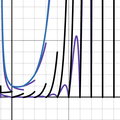
Desmos
And i think i understand why they look different but i dont understand why ceil is much more exact
i may be able to get floor to look like that tho if i tweak it enough
Also this method does converge extremely quickly whith k values of 12 having an error of 0.001
 cunning moat
is this the correct channel for a question about a problem from Finite Elements Method?
cunning moat
or more exactly the theory behind the problem
heady mesa
Yes
heady mesa
rose meteor
Also this method does converge extremely quickly whith k values of 12 having an ...
How are you calculating this error? As x get's larger we would also expect the error between $\Gamma(x)$ and your approximation to get bigger?
pine jettyBOT
Max
 heady mesa
Whenever studying something it's great to find your own way, but perhaps do some research on what other methods people have done and compare. It may be that actually this is quite slow. (Like newton raphson method converges quadratically so in 12 iterations we get a root that is roughly 4096 times as accurate as the first root...)
Also for error, doing some sort of integral might be better? Ie. $$\int_a^b\lvert \Gamma(x)-ApproxOfGamma(x)\rvert dx$$, where $a,b$ is the interval of interest.
pine jettyBOT
Max
 cunning moat
ok so, when we were solving the Poisson equation generally using 2D FEM with linear polynomials, we derived an element-wise computation formula for the local stiffness matrix components that doesnt really depend on the shape function since it uses the transformation to the standart triangle
Similarly when we were on the theory of L2-projection for 2D FEM using linear polynomials a formula was given to us for the local mass matrix components something of the sort $$\frac{|\tau|}{12}*
\begin{matrix}
2 & 1 & 1 \
1 & 2 & 1 \
1 & 1 & 2
\end{matrix}$$
Both of which are firmulas for triangulation mesh
(Im not familiar how the discord bot for TeXiT works so idk if that will render and im a newbie at using LaTeX as a whole)
My question is, why would those formulas not work for solving the wave equation (where its requried to compute both the mass and stiffness matrix) when both of them are independent on the shape functions but only on the type of the mesh (to be triangulation) and on the triangle you are in currently?
pine jettyBOT
HelODeh
 rose meteor
heady mesa
Also for error, doing some sort of integral might be better? Ie. $$\int_a^b\lver...
rose meteor
heady mesa
Also for error, doing some sort of integral might be better? Ie. $$\int_a^b\lver...
Ok wait this is really smart thanks for the help
however
one very strange thing i have noticed
rose meteor
Sorry it took a little bit to test this
but ive noticed that for large values being apporximated
like say the approximation of 216.513!
taking the approximation of like 1.513!
and then scaling it up ith 2.513 * 3.513 * 4.513... and so on until 216.513
there is actually less error in doing it that way then just straight up taking the approximation of 216.513!
which is really starange to me because i dont understand how that could happen unless the error for larger numbers was not proportional to theyre size
 wary oriole
 wary oriole
yes wait a min
    n = a.shape[0]

    for k in range(0, n - 1):
        if a[k, k] == 0:  # stop if pivot is zero
            raise LinAlgError("Singular matrix")
        for j in range(k + 1, n):
            for i in range(k + 1, n):
                m_ik = a[i, k] / a[k, k]  # compute multipliers for current column
                # a[i, k] = m_ik
a[i, j] = a[i, j] - m_ik * a[k, j] # apply transformation to remaining submatrix```so this is my implementation of lu decomp without pivoting. somehow it's not correct. i based my on above algo

this is step by step
my result is
 [ 4 -4 -6]
 [ 4 -2 -1]]```
which is the supposed U. but I can't do L at the same timeso this algo according to bhte book, you are not suppose to store L, or U, instead change U in place in A as upper triangluar including diagonal, L as lower traangluar portion of A, but not including diagonal as it's unit diagonal. so my result is correct in U, but that A[3, 2] should be 0.5 according the hand-calculation.
 [ 4 -4 -6]
 [ 4 0.5 -1]]
this is intended.
how to correct it?
wary oriole
oh I got it. np.array has dtype. if you do
a[i, k] = m_ik```
on a integer matrix, with m_ik = 0.5, numpy will make it 0. Just declare dtype=float gray tundra
here is the iterations for newton raphson method. They are computing relative error in each iterations and i was wondering why is it that eps = (x(k+1)-x(k))/x(k)

my problem with this formula is that i think that the denominator should be the closest value to the real value which is x(k+1)
wide spear

 outer jacinth
im like wondering how to compute both because my teacher isnt very clear
wide spear
wary oriole
Here is an outline
outer jacinth
coding it for me inst the issue i think its more connceputally
wide spear
Well, do you understand gaussian elimination?
outer jacinth
wide spear
Well, do you understand gaussian elimination?
yes kind of essientially isnt the point of it getting it to row echelon form without any swaps or zeros
wide spear
Do you understand how gaussian elimination helps us solve systems of linear equations
 granite aurora
@wide spear you familiar with taylor series and how they help integrate differential equations?
granite aurora
i have a problem that states the following:
derive and explain the method of Taylor series for integrating a differential equation
y' = f(x,y) , y(x0) = y0
Then asks what is the main issue of using this method to integrate such equations
wide spear
This is more appropriate for #odes-and-pdes
granite aurora
it involves ODE but its a numerical method that approximates the integral thats why i thought to ask here first but thanks ill try there as well
outer jacinth
wide spear
Do you understand how gaussian elimination helps us solve systems of linear equa...
i mean not entirely
all ik is u get a answer but im really bad at thinking of things abetrially with math 18
linear algerbra *
outer jacinth
wide spear
By hand
is there any good textbooks or videos i can watch to learn this stuff
wide spear
Any intro linear algebra textbook should cover this
Friedberg Insel Spence is what I used
wide spear
I don't remember
 vast nexus
Hi, how would you solve problems like this?
 wide spear
Numerically?
vast nexus
wide spear
Numerically?
Yes
outer jacinth
is there any good youtube videos on this stuff
im debating if its even possible to get a 60 % in this class
vast nexus
I didn't take good notes in the first couple lectures and I am worried because I can't find resources on our problems 😭
fathom rain
vast nexus
Hi, how would you solve problems like this?
plot and visually pick an interval
vast nexus
fathom rain
plot and visually pick an interval
my professor did not use a graphing calculator in class while solving this but i don't remember his approach
do you know a numerical approach?
fathom rain
test a few values and see where there sign of the functions changes. you can use newton's method to find the roots
vagrant jackal
my guess is that it intends you to evaluate at a bunch of points and note where the sign changes, then go "by IVT there is a solution here"
fathom rain
vast nexus
my professor did not use a graphing calculator in class while solving this but i...
like on the first one, you have different signs for x=0 and x=1
which should tell you something
vast nexus
fathom rain
like on the first one, you have different signs for x=0 and x=1
that's true, so [0, 1] would be a solution?
since f(0) < 0 < f(1)
fathom rain
vast nexus
that's true, so [0, 1] would be a solution?
since f(0) < 0 < f(1)
yes, like cloud said above, ivt: https://en.wikipedia.org/wiki/Intermediate_value_theorem
fathom rain
vast nexus
that's true, so [0, 1] would be a solution?
since f(0) < 0 < f(1)
on b you have 3 roots = 3 sign changes = 3 intervals
brave crypt
Why is discrete 1-d laplacian poorly conditioned
Like its supposed to be O(N^2) but i dont see it immediately, do I have to go thru what row reduction or is there a quciker way
Where N is 1/h
wide spear
brave crypt
Like its supposed to be O(N^2) but i dont see it immediately, do I have to go th...
What is supposed to be O(N^2)?
fathom rain
brave crypt
Why is discrete 1-d laplacian poorly conditioned
it has a zero of order 2, since the spectral symbol is 4sin^2(t/2)
the smallest eigenvalue (dirichlet) is 4sin^2(pi/(2(n+1))) and the largest is 4sin^2(npi/(2(n+1)))
brave crypt
wide spear
What is supposed to be O(N^2)?
Matrix condition number
brave crypt
fathom rain
it has a zero of order 2, since the spectral symbol is 4sin^2(t/2)
Are u supposed to get this with the greens function thing?
Im not exactly sure what a spectral symbol is sorry
fathom rain
spectral symbol describes the eigenvalue distribution. it will also describe haw fast the smallest eigenvalue goes to zero
brave crypt
Ok that sounds important
brave crypt
I would appreciate this thanks!
fathom rain
brave crypt
I would appreciate this thanks!
it is describe for example in here https://link.springer.com/book/10.1007/978-3-319-53679-8
brave crypt
Wow this is cool
);
I lost internet but I have mobile data
Does this book introduce spectral symbols too?
In class we are going to go over spectral methods in more depth
But that doesnt show up until page 300 of the textbook
fathom rain
brave crypt
Does this book introduce spectral symbols too?
yes and for the laplacian you have it for example in remark 10.2
fathom rain
brave crypt
Does this book introduce spectral symbols too?
it is a rather obscure concept for most people. but very powerful
brave crypt
fathom rain
it is a rather obscure concept for most people. but very powerful
Yeah it sounds obscure but it seems like it that would be a lot of information
Its just linear algebra though?
fathom rain
brave crypt
Its just linear algebra though?
yes
brave crypt
Like spectral symbol is probably only relevant for those high dimensional operators
Yeah my book doesnt have anything about spectral symbol
fathom rain
brave crypt
Like spectral symbol is probably only relevant for those high dimensional operat...
it comes from operator theory, i use it for highly efficient and accurate eigenvalue computations
brave crypt
Imma see if trefethens book has it
fathom rain
brave crypt
Imma see if trefethens book has it
probably not
brave crypt
Ok cool
fathom rain
if you look at any book about pseudospectra or structured matrices you will find it
brave crypt
Yeah I dont know if I am ready to formally learn operator theory as I havent taken a class on functional analysis yet
wary oriole
anyone doing FEM has experience with NGSolve? If I want to create a 3by3 squares (like tic tac toe) geometries in 2D do I have to create nice Rectangles? I feel like there is a easier way to do this?
 crisp lake
I'm having a brainfart or something & can't figure out how/why Clenshaw summation works.
crisp lake
No, the efficient method for evaluating finite sums of functions satisfying 3-term recurrences.
crisp lake
wide spear
What don't you understand
It’s described in this paper if you can grasp it & somehow explain it to me: https://www.ams.org/journals/mcom/1955-09-051/S0025-5718-1955-0071856-0/S0025-5718-1955-0071856-0.pdf
wide spear
Is there a specific part that you don't understand
crisp lake
wide spear
Is there a specific part that you don't understand
The proof of why the method is correct. I guess I don't follow the penultimate line «Then application of the recurrence relation (6) shows that…» and the final equation.
wide spear
Ok I would first try to understand why this works for just chebyshev polynomials as shown in equations 1-3
In particular, pick some A_n and compute the sum directly and using the reversed recurrence relation by hand
molten knot
wary oriole
anyone doing FEM has experience with NGSolve? If I want to create a 3by3 squares...
the way I do it is set the endpoints and draw lines between them
and then set an index inside and out to denote the boundary
there might be an easier way tho
crisp lake
wide spear
In particular, pick some A_n and compute the sum directly and using the reversed...
I just tried that & must have miscalculated or something because the results didn't line up.
wide spear
Well, let's see the calculation
crisp lake
$2\cdot T_0(x)+3\cdot T_1(x)+5\cdot T_2(x)+7\cdot T_3(x)$ was what I just tried.
pine jettyBOT
Nadia
 crisp lake
wide spear
Well, let's see the calculation
crisp lake
wide spear
Well, let's see the calculation
I actually did it on Microsoft whiteboard on my iPad Mini, so in principle, there should be some way to capture it.
crisp lake
Here:
 crisp lake
I'll give it another shot.
crisp lake
I got it wrong again.
pine jettyBOT
Angetenar
 wide spear
The reverse recurrence gives $B_4=B_3=0$, $B_2=A_2$, $B_1=A_1+(4x-2)B_2=A_1+(4x-2)A_2$, and $B_0=A_0-B_2+(4x-2)B_1=A_0-A_2+(4x-2)A_1+(4x-2)^2A_2$ right?
pine jettyBOT
Angetenar
 wide spear
So in theory, $f(x)=B_0-(2x-1)B_1=A_0-A_2+(4x-2)A_1+(4x-2)^2A_2-(2x-1)A_1-(2x-1)(4x-2)A_2$
pine jettyBOT
Angetenar
 wide spear
And using $2x-1=\cos\theta$ and grouping like terms, this becomes $A_0+A_1\cos\theta+A_2(2\cos^2\theta-1)$
pine jettyBOT
Angetenar
 wide spear
Which is correct
crisp lake
I'm getting wrong answers repeating this in Maxima.
wide spear
Do you understand the computation I did at least
crisp lake
Yes, something is going seriously awry in my hand calculations.
wide spear
Hopefully you figure that out
Now as to the intuition as to why this works
As we perform the reverse recursion down to n=0, we use the recurrence relation that defines the T_n right
So like if we look at the A2 part
We start with A2, then (4x-2)A2, then (4x-2)^2A2-A2
Which recursively builds up T2
crisp lake
wide spear
Hopefully you figure that out
Still unsure why it's not working.
wide spear

crisp lake
wide spear
Hopefully you figure that out
There is the maxima file.
wide spear
I don't know maxima
crisp lake
What's done there is trivial enough that it shouldn't be an issue.
wide spear
I think the only issue might be the expansions of FA vs FB
crisp lake
I'm not sure what you mean.
crisp lake
wide spear
I think the only issue might be the expansions of FA vs FB
The Chebyshev polynomials are shifted i.e. $T^*_n(x)=T_n(2x-1)$.
pine jettyBOT
Nadia
 crisp lake
wide spear
I think the only issue might be the expansions of FA vs FB
crisp lake
wide spear
I think the only issue might be the expansions of FA vs FB
The updated maxima file:
wide spear
Is it correct?
crisp lake
wide spear
Is it correct?
The two match now. The problem was that the example in Clenshaw's paper used the recurrence coefficients for $T^*_n(x)=T_n(2x-1)$ and I was using the recurrence coefficients for $T_n(x)$. When I used a consistent set of recurrence coefficients for a consistent orthogonal polynomial basis it all worked.
pine jettyBOT
Nadia
 wide spear
Ok nice
Did the example I worked by hand help to provide some intuition about why clenshaw works?
crisp lake
wide spear
Did the example I worked by hand help to provide some intuition about why clensh...
I should probably do a similar exercise instead of using a concrete orthogonal polynomial basis.
wide spear
Sure
But doing some calculations by hand should provide some insight into why it works
crisp lake
I think there should be an orthogonal polynomial product formula like $\phi_{m}(x) \phi_{n}(x)=\sum_{k=0}^{mn}\alpha_{k}\phi_k(x)$ out there somewhere but am not finding generalisations of what I see for e.g. Chebyshev polynomials.
pine jettyBOT
Nadia
 heady mesa
If you want to come up with one for Chebyshev polynomials then use: $T_n(\cos \theta)=\cos(n\theta)$
pine jettyBOT
Max
 heady mesa
I think the result you are looking for follows pretty quickly when you use product of sum, ie.
 crisp lake
heady mesa
If you want to come up with one for Chebyshev polynomials then use: $T_n(\cos \t...
crisp lake
heady mesa
If you want to come up with one for Chebyshev polynomials then use: $T_n(\cos \t...
I have the one for Chebyshev polynomials and am hoping for a more general version for orthogonal polynomials.
heady mesa
I doubt it exists
crisp lake
heady mesa
I doubt it exists
I'm willing to take restrictions on the class of orthogonal polynomials.
heady mesa
Things in general are really tricky, Chebyshev polynomials have some super nice identities and follow nice rules, generalizing them to even really nice and well known orthogonal polynomials such as Laguerre polynomials is usually unfruitful
wide spear
Yeah I'm not aware of any such product formulas even for the Legendre polynomials
crisp lake
I think Legendre have them.
Maybe it's Sturm-Liouville eigenfunctions, maybe it's some kind of umbral calculus. It's tougher to use the things as a basis without being able to take products.
wide spear
I'm not sure I agree
I very rarely need to multiply elements of a basis
Unless I'm taking an inner product of two functions in which case I don't want to explicitly multiply them either
crisp lake
For my purposes I do need multiplication.
wide spear
What are you trying to do?
crisp lake
wide spear
What are you trying to do?
These guys are representing probability densities with splines that are in plain monomial form, so the alternative strategy I'm thinking about is being able to represent the splines' polynomial pieces in a basis that facilitates taking expectations using the modelled density.
One of the tasks they do is computing a centile histogram.
wide spear
By splines you mean a bunch of polynomials of degree n on intervals with some continuity/differentiability condition at the endpoints right
If you're working with splines, sort of the natural basis to work with are the Bernstein polynomials
crisp lake
I can't actually tell how they're computing the spline to represent the probability density. I might be missing how their code is getting invoked because it's mostly the centile histogram root-finding.
crisp lake
wide spear
If you're working with splines, sort of the natural basis to work with are the B...
Not M-splines?
wide spear
Well now it depends on what types of splines are being used
crisp lake
(Basically B-splines renormalised to integrate to 1.)
wide spear
Spline is very overloaded
Anyways are chebyshev polynomials not satisfactory for some reason
crisp lake
wide spear
Anyways are chebyshev polynomials not satisfactory for some reason
Maybe ignoring the orthogonal polynomials for a moment, they're trying to do Descartes' rule of signs or Vincent's and need to do $(cx+d)^{\deg p}p\left(\frac{ax+b}{cx+d}\right)$ efficiently somehow. Or at minimum a translation $p(x+a)$.
pine jettyBOT
Nadia
 crisp lake
Quantile histograms for distributions with densities given by splines, basically.
wide spear
Is direct evaluation too slow?
crisp lake
wide spear
Is direct evaluation too slow?
I'm not sure if it's a performance hot path or anything, but they (and I) seem to be adrift from much grounding in literature/theory/etc.
crisp lake
Still looking around for more quantile algorithms for distributions whose densities are represented by splines.
I'm pretty sure that their spline density functions are empirically determined but I have no idea how, so there's some weirdness about dynamically updating the quantile histograms as new samples are acquired.
crisp lake
Schumaker (2007) has Chebyshev splines and gives Budan-Fourier theorems for polynomials in the Chebyshev basis.
brave crypt
Hi is there anyone familiar with nonlinear parabolic pde?
crisp lake
This can't be right. Somehow 1D Newton with bracketing interval & fallback to bisection has nowhere obvious to look it up.
wide spear
What do you mean look it up
crisp lake
wide spear
What do you mean look it up
When I look up Newton's method I don't see more stuff about how it's plugged into frameworks to stay within bracketing intervals, detect multiple root issues etc.
wide spear
I mean you can find an implementation of newton's method and see how they do it
But there's really not that much to it
molten knot
crisp lake
When I look up Newton's method I don't see more stuff about how it's plugged int...
aren’t multiple roots just handled by sampling lots of initial conditions
crisp lake
molten knot
aren’t multiple roots just handled by sampling lots of initial conditions
I believe that Newton deals with n-fold roots by an integer factor in the denominator of the update.
 meager dome
(I´m not sure if this questions goes here or in the cs channel!)
Hey! I have a doubt about some methods we have been using for proving some elementary bounds in a introductory numerical analysis class.
For example, we made bounds for the relative error of calculating a^3b with a, b numbers of the machine that were like 3\eps + O(\eps^2); in the proof we use constantly that x* = x(1 + \delta) (being x* the rounding of x as a number of the machine), and we use it operation by operation, i.e:
a^3b => ( ((a^2)* a)* b )* = ( ((a^2)(1 + \delta_1) a)* b )* = ( ((a^3(1 + \delta_1)(1 + \delta_2) b )* = a^3b(1 + \delta_1)(1 + \delta_2)(1 + \delta_3)
And for this we get the bound, knowing that |\delta_i| \leq \eps.
It was said in the class that one could "replace the operation in the machine with the real operation times a factor (1 + \delta)" with every normal operation except with substracting, and that this was related to the known catastrophic cancellation that happens when you substract similar numbers.
I get that with catastrophic cancellation in mind you have the fact that there is no good bound for substracting numbers in a machine, but I do not get how to precisely formalize the idea that if you want to multiply, sum or divide machine numbers you have a good bound (and you can operate like before) but with the substracting you can´t.
Any advice or resource would be helpful.
wide spear
Have you seen the proof of the sterbenz lemma
meager dome
No, thx for mentioning it. It seems useful for the doubts I have.
 minor vigil
guys, anyone knows if there exists an efficient way to compute the full QR decomposition?
more specifically, if there exists clever way to obtain an orthogonal basis of Nu(A^T)
the reason for my question is because you can always obtain an orthogonal basis for the orthogonal complement of a single vector using house holder transformations
wide spear
There exist efficient QR algorithms, yes
minor vigil
$Rx= e_1 \Rightarrow R^2x = Re_1 \Rightarrow x = Re_1$
pine jettyBOT
jeca tatu
 minor vigil
where R is the householder reflection matrix
wide spear
One method is indeed based on householder reflections
minor vigil
and because R is orthogonal and R_1 = x, then all the other columns form a basis for the orthogonal complement of x
ok, but the full QR requires obtaining a basis for Nu(A^T) right?
I dont know if theres a clever way to do that without much effort
wide spear
How efficient of an algorithm do you want
minor vigil
something like to obtain an orthogonal basis for span{v1,...,vk} and get the complement for almost free
I dont know if thats possible
wide spear
Practically speaking, all QR decomposition algorithms will be O(n^3) unless your matrix is structured in some way
minor vigil
hmm
I just find curious how you can obtain the orth. complement of a single vector in a easy way
and I suspect that this trick could work for a collection of more vectors
wide spear
What does easy mean to you
minor vigil
I dont know, really
I just wanna know if it is at least something that can be visualized by some operations after performing householder to the set
Ill try to investigate it a little bit more
in the case of 1 vector the result is trivially by construction of the reflection of the first vector always to a multiple of e1
but for the subsequent operations you kinda look to the submatrices and things gets more complicated

 weak gyro
pls help <@&286206848099549185>
 thorny pulsar
what is the best introductory book on numerical analysis (preferably at the graduate level) that is a good mix of theory and application?
wide spear
Are you looking for numerical linear algebra or numerical differential equations or numerical optimization or something else
thorny pulsar
honestly a bit of everything, nla, diff eq, integration differentiation, rootfinding, polynomial interpolation
if you have multiple book reccs I wouldn't mind
wide spear
There is an introductory textbook to numerical analysis, Burden and Faires, but I would say that it is at the undergraduate level
For grad level books, they are generally specialized into one of the specific areas that I mentioned
E.g. Demmel for numerical linear algebra and Iserles for numerical differential equations
thorny pulsar
okay thanks, I'll check them out
 next garden
Does anyone know a good introductory text on the Diffuse element method / Diffuse Approximation ?
fathom rain
next garden
Does anyone know a good introductory text on the Diffuse element method / Diffus...
this seems to be the first hit and mostly cited https://link.springer.com/article/10.1007/BF00364252 any reason to use this? (probably pretty obscure method?)
fathom rain
next garden
Does anyone know a good introductory text on the Diffuse element method / Diffus...
sounds a bit like RBF:s?
wide spear
RBFs + moving least squares it seems to me
next garden
fathom rain
this seems to be the first hit and mostly cited https://link.springer.com/articl...
I am trying to find a robust way of computing the principal curvatures and principal directions of a smooth manifold defined as an SDF
So I am trying to find robust numerical ways of getting the partial derivatives
next garden
fathom rain
this seems to be the first hit and mostly cited https://link.springer.com/articl...
This is the original paper. But papers are usually much harder to understand, I was hopping for a textbook chapter or course notes. Those tend to be much more digestible.
Alternatively the paper i am currently reading suggests using lagange differentiation
fathom rain
no idea, never heard of this before
next garden
fair enough, thank you for the help still
wide spear
What techniques have you tried and deemed unsuitable?
next garden
regular finite differences (centered)
it's too unstable
too sensitive to the h parameter (the spacing)
wide spear
Hmmm did you try regular finite element
Or a voronoi method
Or a triangularization/spline based method
fathom rain
iga
 undone nebula
crisp lake
When I look up Newton's method I don't see more stuff about how it's plugged int...
undone nebula
crisp lake
When I look up Newton's method I don't see more stuff about how it's plugged int...
I read your messages, are you trying to find real roots of a polynomial? I have an implementation on my GitHub which uses continued fractions if you need, it’s in TypeScript
It doesn’t have arbitrary precision or exact arithmetic though but you can just makes some changes if you need numerical stability
I went down a super deep rabbit hole on this too
next garden
wide spear
Hmmm did you try regular finite element
I don't have a mesh so direct FEM won;t work. I am actually tring to triangluate the isosurface with a new method, so any method that relies on a mesh is redundant.
What is a voronoi mehtod? That is new to me? Can you offer an exmaple/resource?
wide spear
Generate a voronoi triangulation of your surface, then use that triangulation to do things
next garden
wide spear
Generate a voronoi triangulation of your surface, then use that triangulation to...
How do you generate a voronoi triangulation of an implicit?
wide spear
In what form is the SDF given to you?
Is it a function that you can evaluate wherever you want?
next garden
wide spear
Is it a function that you can evaluate wherever you want?
Yes, it;s a funciton pointer
so just some f(x,y,z)
that returns a scalar
wide spear

arXiv.org
Volumetric shape representations have become ubiquitous in multi-view reconstruction tasks. They often build on regular voxel grids as discrete representations of 3D shape functions, such as SDF or radiance fields, either as the full shape model or as sampled instantiations of continuous representations, as with neural networks. Despite their pr...
 green folio
Bit of a long shot, but does anyone know how compute peak indexing for a sample that exhibits multiple bravais lattice structures in GSAS-II (or any other refinement software)
 versed marsh
Let $-\pi \leq \theta \leq \pi$. The sequence $S_n = { sin(\theta)}$. This is an example of a bounded sequence but not a Cauchy Sequence?
pine jettyBOT
Ashp116
 versed marsh
The sequence $S_n = { 1/xsin(x)}$ is a Cauchy Sequence? If so, it is not monotonic right?
pine jettyBOT
Ashp116
 wide spear
next garden
wide spear
next garden
Question In this document, section 2.2 talks about a technique called lagrange differentiation. I have not heard about this concept before (although it seems to come from a generalization of lagrange polynomials to higher dimensions).
I was hoping someone here would have so pointers to other resources. The mentioned paragraph doesn;t seem to have a reference to anything.
fathom rain
next garden
Question In this document, section 2.2 talks about a technique called lagrange d...
lagrange interpolation and then take derivatives of those
next garden
fathom rain
lagrange interpolation and then take derivatives of those
I don't think it is quite that. If you look at the coefficients. There is no parameter. It entirely yields constants.
So at minimum it has to be evaluating the parameters somehow.
It's also multiplying multiple basis together.
wide spear
What about the paragraph is unclear
next garden
This is not directly a lagrange polynomial. It is similar, but note how the numerator does not have a difference, it's just a constant. (Similar to the others)
And then look at the application of the polynomials. There is no paramater, the direct derivative of a lagrange polynomial would have a parameter. So at most this is taking the derivative of a LP and then evaluating its derivative at a fixed parameter


that's the only way I can think of where you would get a constant
next garden
Not sure, I am tempted to say it is x=0 because then it would explain why the numberator is only the constants
however nrmally LPs start at 0 on the first knot
which is not what's happening here
that's why I am confused
wide spear
Are you confusing Lagrange polynomials with splines
next garden
no
wide spear
Lagrange interpolation does not have any parameters
next garden
wide spear
Lagrange interpolation does not have any parameters
?
https://en.wikipedia.org/wiki/Lagrange_polynomial
Any interpolation will have a parameter, because your input set you are interpolating over is just a point set

In numerical analysis, the Lagrange interpolating polynomial is the unique polynomial of lowest degree that interpolates a given set of data.
Given a data set of coordinate pairs
    (

      x

        j


    ,

      y

        j
...
to get in betweens you need to blend them
for that you need a parameter
 wide spear
No, you weight the basis according to the values at the interpolation points and add them
Which one of those is a parameter
wide spear
The xi are the interpolation points
wide spear
Ok that’s not how we use the term parameter
next garden
That's how it was used in the classes I took
parametric curves are called parametric curves because they take a parameter
wide spear
Ok whatever
next garden
the parameter being the free variable that allows you to interpolate
So the reason why I am confused with the text is precisely because that free variable/parameter is missing
so it should have been evaluated somehwere
wide spear
If I understand the text correctly, that is over a stencil with a fixed grid spacing delta x
next garden
but the text doesn;t say to what
wide spear
It gives the derivative values the grid points
next garden
wide spear
It gives the derivative values the grid points
Yes, but if you were to evaluate any of the lagrange basis polynomials at a given grid point, you would have a difference in the numerator

so that $b_{ik}$ should instead be something like $b_{ik} - b_{im}$
pine jettyBOT
Makogan
 next garden
like if oyu just grab the definition of a lagrange basis polynomial and evaluate it to a given point in space you get differences in the numerator
wide spear
Yes, the b_ik are differences
After 10c, for example, it says that b_i1=-delta x, bi2=0, and bi3=delta x
next garden
wide spear
Yes, the b_ik are differences
Yes, but that's only for the specific example given. I assume that you can express them as relative offsets from the pint at which you are taking hte derivative
 river thicket
does anyone know that if i have
minimize $_\beta \vert \vert A \beta - y \vert \vert^2$
pine jettyBOT
Jonathan
 river thicket
and A is a compex matrix
if the solution is:
$\beta = (A^A)^{-1}A^ y$
where A^* is the conjugate transpose matrix of A ?
pine jettyBOT
Jonathan
 wide spear
Yes
 neat haven
$\frac{dP(r)}{dr} = -\frac{G}{r^2}\left[\rho(r) + \frac{P(r)}{c^2}\right] \left[M(r) + 4\pi r^3 \frac{P(r)}{c^2}\right] \left[1 - \frac{2GM(r)}{r c^2}\right]^{-1},$
pine jettyBOT
Farm
 neat haven
pine jetty
**Farm**
neat haven
pine jetty
**Farm**
Hello, I'm trying to solve the Tolman–Oppenheimer–Volkoff equation for modeling a neutron star using a polytropic equation of state of the form
What numerical method is recommended for integrating these equations? I've heard that Runge-Kutta methods are commonly used, but I'm not sure how to deal with the stiffness that might arise in the equations, especially near the center.
Sorry if this isn't the correct channel, but it is one of the most active.
-using a polytropic equation of state of the form
$P = K \rho^{\gamma},$
pine jettyBOT
Farm
 wide spear
Have you tried anything yet
If you haven't, start with RK4
If you have stiffness issues, then come back and we can discuss more
neat haven
I started with addressing the singularity at $r = 0$, then I tried to derive a Taylor series expansion for $M (r) and P (r) near R = 0$ and used the approximations for a small, non-zero radius. But really that's all.
I eventually added a standard fourth-order Runge-Kutta method to integrate the TOV equations. However, I've encountered some problems in the results that suggest there might be errors introduced when I used the method.
pine jettyBOT
Farm
 wide spear
Hmmmm
What happens if instead of integrating from 0 to r_1 you integrate from eps to r_1
Prescribing an initial condition for P(eps)
What problems are there in the results?
 violet sundial
I'm trying to figure out how to get the orientation of a face-transitive polyhedron given a rotation matrix. Specifically, I'm thinking dice (beyond just 6-sided). If I label each face in some starting orientation and calculate normals for each face, I could rotate the normals once the polyhedron itself is rotated and find one which is pointing roughly "up", but that gets to be a lot of work as the number of faces increases. Is there some other method I'm missing?